Statistics Manual of Haidian Foreign Language School
May 19, 2026
Preface
Welcome to the Statistics Manual of Haidian Foreign Language School — a project-based introduction to statistics using R.
This book is designed for students with no prior experience in statistics or programming. If you can use a web browser, you have all the technical background you need to get started.
0.1 What Is Statistics?
Every day, you are surrounded by data. Your phone tracks your screen time. Weather apps predict tomorrow’s temperature. News headlines report that “72% of surveyed residents support the new policy.” All of these are examples of statistics in action.
Statistics is the science of collecting, analyzing, and drawing conclusions from data. At its core, it is a process:
- Collect data.
- Summarize the data so you can understand it.
- Interpret the results to draw meaningful conclusions.
That is the entire discipline, distilled to three steps. Everything we do in this book — every chart, every test, every line of R code — serves one of these three goals.
But why should you care? Because statistics gives you the power to move from opinion to evidence. Instead of saying “I think most students prefer morning classes,” you can survey 200 students, summarize the responses, and state a conclusion backed by data. That skill — turning raw information into useful knowledge — is valuable in every field, from medicine to business to environmental science.
0.2 A Project-Driven Approach
This book is organized around a single idea: statistics in the service of questions.
Rather than memorizing formulas in isolation, you will choose a research question that genuinely interests you and pursue it across every chapter. You might ask:
- Is there a relationship between sleep duration and academic performance?
- Do left-handed and right-handed people differ in reaction time?
- Can a country’s GDP per capita predict its life expectancy?
The question you pick will drive every analysis you do. When we learn about frequency tables, you will build one for your variables. When we learn about hypothesis testing, you will run a test on your data. By the final chapter, you will have completed an entire research project — from question to conclusion — that you can present with confidence.
By working through this book, you will learn to:
- Generate testable research hypotheses
- Understand and navigate large, real-world datasets
- Manage and format data using R
- Conduct both descriptive and inferential statistical analyses
- Present your results clearly to any audience
0.3 Population and Sample
Before we can collect data, we need to know who or what we are studying. In statistics, the word population refers to the entire group we want to learn about. A population could be:
- All students at a high school in Beijing
- All smartphones manufactured by a company in 2025
- All lakes in a national park
In most real situations, the population is far too large to study completely. You cannot survey every student in China, test every smartphone off the assembly line, or sample every lake. Instead, you study a sample — a smaller subset of the population.
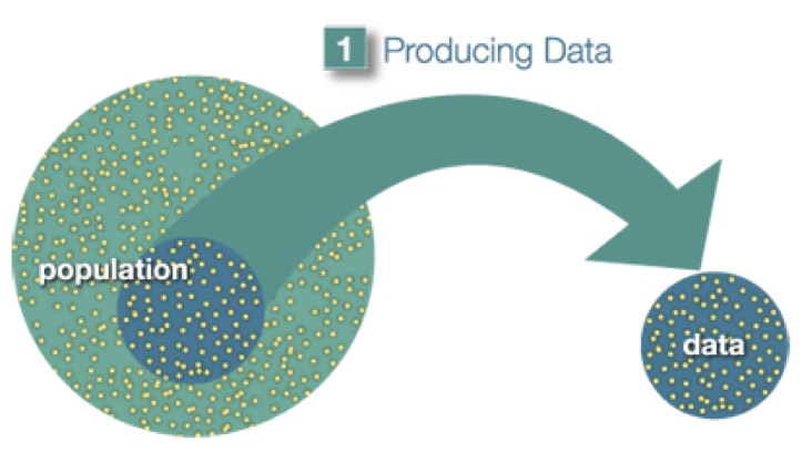
Figure 0.1: A sample is a subset drawn from the population.
Here is the key insight: if the sample is chosen well, it can represent the population. A sample of 1,000 randomly selected high school students in Beijing can tell you something meaningful about all high school students in Beijing — but only if the sample is not biased toward one school, one district, or one income level.
0.4 The Big Picture of Statistics
Statistical work follows a clear pipeline. Think of it as three stages:
Stage 1 — Producing Data. You choose a sample from the population and collect information from it. This might mean conducting a survey, running an experiment, or downloading an existing dataset.
Stage 2 — Exploratory Data Analysis (EDA). Once you have the data, you summarize and visualize it. How are the values distributed? Are there outliers? What patterns emerge? EDA is about getting to know your data before you make any formal claims.
Stage 3 — Inference. Finally, you use what you learned from the sample to draw conclusions about the population. Because the sample is only a subset, there is always some uncertainty — inference is the toolkit for quantifying that uncertainty and making defensible claims.
0.4.1 A Concrete Example
In April 2005, ABC News and the Washington Post conducted a poll about U.S. adults’ opinions on the death penalty. Here is how the three stages played out:
- Producing Data. A representative sample of 1,082 U.S. adults was selected and asked whether they favored or opposed the death penalty.
- Exploratory Data Analysis. 65% of the sampled adults favored the death penalty.
- Inference. The pollsters concluded — with 95% confidence — that the true percentage of all U.S. adults who favored the death penalty was between 62% and 68%.
Notice the flow: collect → summarize → generalize. Every statistical study follows this pattern.
Because this book uses datasets that have already been collected, our focus will be on Stage 2 (EDA) and Stage 3 (Inference). You will not need to design your own survey or run your own experiment — the data is waiting for you. Your job is to explore it, analyze it, and tell a story with it.
0.5 How This Book Works
Chapters are organized into four parts:
- Part I — Foundations: What data looks like and how to manage it
- Part II — Exploratory Data Analysis: Visualizing and summarizing your data
- Part III — Statistical Inference: Testing hypotheses and drawing conclusions
- Part IV — Modeling: Building more complex analyses
EDA chapters use a TL;DR → Deep Dive format: a quick, code-forward summary you can use immediately, followed by the full explanation. Inference and modeling chapters use a Motivating Example → Theory → Code → Interpretation format, walking you through a real analysis from start to finish.
You will work with a single dataset throughout the book, building your analysis chapter by chapter. By the end, you will have completed an entire research project — from question to presentation.
0.6 Getting Started with R and RStudio
Throughout this book, you will use R — a free, powerful programming language for statistics — and RStudio — a user-friendly interface for working with R. Think of R as the engine and RStudio as the dashboard. When you sit down to work, open only RStudio — not the R application. RStudio runs R silently in the background. You never need to open R directly.
0.6.1 Installing R
- Go to https://cran.r-project.org/.
- Click the link for your operating system (Windows, macOS, or Linux).
- Download the latest version and run the installer.
- Follow the default options.
0.6.2 Installing RStudio
- Go to https://posit.co/download/rstudio-desktop/.
- Download the free RStudio Desktop version for your operating system.
- Run the installer with the default settings.
You must install R before RStudio. RStudio needs R to function.
0.6.3 The RStudio Interface
When you first open RStudio, you will see four panels:
- Source (top-left): Where you write your code and R Markdown documents.
- Console (bottom-left): Where R runs your code and displays results.
- Environment (top-right): Shows the data and objects you have loaded.
- Files / Plots / Help (bottom-right): Browse files, view charts, and read documentation.
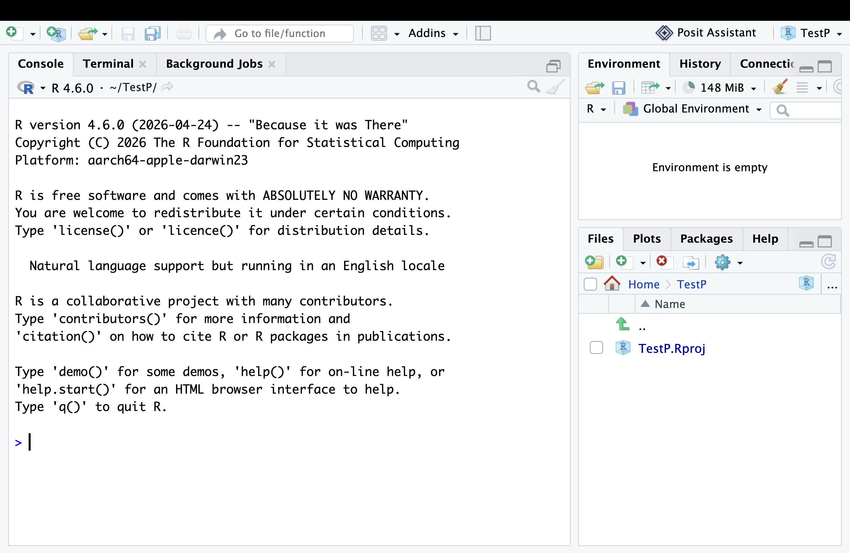
Figure 0.2: The RStudio interface with its four main panels.
0.6.4 Your First R Commands
Let’s try some basic arithmetic. In the Console panel, type the following and press Enter:
## [1] 2R evaluates the expression and prints the result. Try a few more:
## [1] 3.333333## [1] 1024## [1] 12The [1] printed before each answer is R’s way of numbering the output — it tells you this is the first (and only) value in the result. It is not an error code. If R prints a long list of numbers, you will see [1] at the start of each new line, helping you count positions.
R works like a powerful calculator. But it can do far more — store data, create plots, run statistical tests, and generate entire reports. You will learn all of this step by step.
0.6.5 Installing the Packages You Need
R packages are add-ons that extend R’s capabilities — like apps on a phone. You download each one once, then open it whenever you need it.
Important: install.packages() is like downloading an app — do it once. library() is like opening the app — you must run it every time you open RStudio. If you skip library() and try to use a package’s functions, R will tell you it cannot find them.
Install the packages you will need throughout this book by running this in the Console:
You only need to run that command once. After that, load the packages with library() at the start of each RStudio session:
0.7 What’s Ahead
This book has 12 chapters. Here is your roadmap:
| Chapter | Topic | What You Will Learn |
|---|---|---|
| 1 | Data Fundamentals | Types of variables, data structures, reading data into R |
| 2 | Univariate Analysis | Frequency tables, measures of center and spread, histograms |
| 3 | Data Management | Filtering, sorting, grouping, and transforming data with R |
| 4 | Bivariate Analysis | Comparing two variables — bar charts, boxplots, scatterplots |
| 5 | Hypothesis Testing | The logic of tests, p-values, and making decisions with data |
| 6 | ANOVA | Comparing means across multiple groups |
| 7 | Chi-Square Tests | Testing relationships between categorical variables |
| 8 | Correlation | Measuring the strength of linear relationships |
| 9 | Linear Regression | Fitting lines to data and making predictions |
| 10 | Multiple Regression | Using several predictors at once |
| 11 | Moderation & Extensions | Exploring more complex relationships |
| 12 | Epilogue | Presenting your project and next steps |
You do not need to understand all of these terms right now. By the time you reach each chapter, you will have the foundation to tackle it. The journey is cumulative: each chapter builds on the last.
Turn the page, and let’s begin with data.