Chapter 6 ANOVA — Comparing Groups
6.1 TL;DR: ANOVA
- ANOVA (Analysis of Variance) extends the t-test to three or more groups. Instead of asking “are these two means different?” it asks “are these \(k\) means all the same?”
- The test statistic is F — the ratio of variation between groups to variation within groups. A large F means the differences between groups are big relative to the natural spread within each group.
- The null hypothesis (\(H_0\)) is that all group means are equal: \(\mu_1 = \mu_2 = \cdots = \mu_k\). The alternative (\(H_a\)) is that at least one mean differs.
- If the ANOVA is significant (p < 0.05), follow up with Tukey’s HSD post hoc test to find which specific pairs of groups differ. Never run multiple t-tests — you will inflate your Type I error rate.
- Effect size matters. Report η² (eta-squared) — the proportion of total variation in the response explained by the group differences — and Cohen’s d for pairwise comparisons.
- The 4-step process from Chapter 5 still applies: (1) state hypotheses, (2) choose ANOVA, (3) assess evidence with F and p-value, (4) draw a conclusion.
# Load packages — install once with install.packages(c("dplyr", "ggplot2", "modelsummary", "broom"))
library(dplyr)        # for filter(), rename(), select(), %>%
library(ggplot2)      # for graphing
library(modelsummary) # for professional summary tables

# Load and prepare the NESARC dataset — same subset from Chapter 3
# ← REPLACE: your file path and filter conditions
NESARC <- read.csv("NESARC.csv")

nesarc <- NESARC %>%
  filter(
    S3AQ1A == 1,         # smoked 100+ cigarettes in lifetime
    S3AQ3B1 == 1,        # smoked in the past 12 months
    CHECK321 == 1,       # valid nicotine dependence data
    AGE <= 25             # young adults only
  ) %>%
  rename(
    Ethnicity          = ETHRACE2A,     # ethnicity (categorical, 1–5)
    Age                = AGE,           # age in years (quantitative)
    MajorDepression    = MAJORDEPLIFE,  # lifetime depression (categorical, 0/1)
    TobaccoDependence  = TAB12MDX,      # nicotine dependence (categorical, 0/1)
    DailyCigsSmoked    = S3AQ3C1,       # cigarettes per day (quantitative)
    Sex                = SEX            # sex (categorical, 1/2)
  ) %>%
  select(Ethnicity, Age, MajorDepression, TobaccoDependence, DailyCigsSmoked, Sex)

# Recode missing values — 99 means "Unknown" in the NESARC code book
nesarc$DailyCigsSmoked[nesarc$DailyCigsSmoked == 99] <- NA    # ← REPLACE: your NA codes

# Label categorical variables — output shows names, not numbers
nesarc$Ethnicity <- factor(nesarc$Ethnicity,                               # ← REPLACE: your variable
  levels = c(1, 2, 3, 4, 5),                                              # the numeric codes
  labels = c("Caucasian", "African American", "Native American",            # ← REPLACE: your labels
             "Asian", "Hispanic"))
nesarc$MajorDepression <- factor(nesarc$MajorDepression,                   # ← REPLACE: your variable
  labels = c("No Depression", "Yes Depression"))
nesarc$TobaccoDependence <- factor(nesarc$TobaccoDependence,               # ← REPLACE: your variable
  labels = c("No Dependence", "Nicotine Dependence"))
nesarc$Sex <- factor(nesarc$Sex, labels = c("Female", "Male"))            # ← REPLACE: your labels

# One-way ANOVA — ← REPLACE: quant_var ~ cat_var,   data = your_data_frame
anova_result <- aov(DailyCigsSmoked ~ Ethnicity, data = nesarc)  # compare means across ethnic groups
summary(anova_result)                                              # view the full ANOVA table
## Df Sum Sq Mean Sq F value Pr(>F)
## Ethnicity 4 6379 1594.7 22.68 <2e-16 ***
## Residuals 1310 92098 70.3
## ---
## Signif. codes: 0 '***' 0.001 '**' 0.01 '*' 0.05 '.' 0.1 ' ' 1
## 5 observations deleted due to missingness# Tukey's HSD post hoc — find which specific groups differ
TukeyHSD(anova_result) # all pairwise comparisons with adjusted p-values## Tukey multiple comparisons of means
## 95% family-wise confidence level
##
## Fit: aov(formula = DailyCigsSmoked ~ Ethnicity, data = nesarc)
##
## $Ethnicity
## diff lwr upr p adj
## African American-Caucasian -4.6786122 -6.603653 -2.753571 0.0000000
## Native American-Caucasian -1.1884161 -5.443508 3.066676 0.9411184
## Asian-Caucasian -5.4444444 -8.876816 -2.012073 0.0001540
## Hispanic-Caucasian -4.5271548 -6.254291 -2.800018 0.0000000
## Native American-African American 3.4901961 -1.045382 8.025774 0.2197360
## Asian-African American -0.7658323 -4.540330 3.008666 0.9814275
## Hispanic-African American 0.1514573 -2.182779 2.485694 0.9997793
## Asian-Native American -4.2560284 -9.608305 1.096248 0.1909569
## Hispanic-Native American -3.3387387 -7.793925 1.116448 0.2442025
## Hispanic-Asian 0.9172896 -2.760217 4.594796 0.9605024Key interpretation: The ANOVA tests whether mean daily cigarette consumption differs across the five ethnic groups. The F-statistic and p-value tell you if any differences exist. If p < 0.05, TukeyHSD tells you which specific pairs of groups are significantly different. Always report effect size (η²) alongside the p-value — it tells you how much ethnicity actually matters.
6.2 Deep Dive: ANOVA
6.2.1 Motivating Example
In Chapter 5, you learned to compare the means of two groups using a t-test. You asked: “Do young adult daily smokers with depression smoke more cigarettes per day than those without depression?” That is a two-group comparison — depression (yes/no) versus a quantitative outcome.
But what if your research question involves three or more groups? For example:
Does the number of cigarettes smoked per day differ across ethnic groups among young adult daily smokers?
You have five groups — Caucasian, African American, Native American, Asian, and Hispanic. You could run t-tests comparing every pair: Caucasian vs. African American, Caucasian vs. Native American, and so on. That would require \(\binom{5}{2} = 10\) separate t-tests. The problem? Every t-test has a 5% chance of a false positive. Run 10 tests, and your overall chance of making at least one Type I error balloons to roughly \(1 - (1 - 0.05)^{10} \approx 0.40\) — a 40% chance of claiming a difference exists when it does not.
ANOVA solves this problem. It gives you a single test that asks: “Are all five group means equal?” If the answer is no, a follow-up procedure — called a post hoc test — identifies which specific pairs differ, while controlling the overall Type I error rate.
Let us set up the data and see what we are working with.
# Load the packages you need for this chapter
library(ggplot2)      # for all graphing
library(dplyr)        # for filter(), rename(), select(), %>%
library(modelsummary) # for professional summary tables

# Load the NESARC survey (43,093 adults) — ← REPLACE: your file path
NESARC <- read.csv("NESARC.csv")

# Build the subset we use throughout the book:
# young adult (<= 25) daily smokers with valid nicotine data
# ← REPLACE: adapt filter, rename, factor labels to YOUR dataset
nesarc <- NESARC %>%
  filter(
    S3AQ1A == 1,         # smoked 100+ cigarettes in lifetime
    S3AQ3B1 == 1,        # smoked in the past 12 months
    CHECK321 == 1,       # valid nicotine dependence data
    AGE <= 25             # young adults only
  ) %>%
  rename(
    Ethnicity          = ETHRACE2A,     # ← REPLACE: rename to meaningful names
    Age                = AGE,           # age in years
    MajorDepression    = MAJORDEPLIFE,  # lifetime depression diagnosis
    TobaccoDependence  = TAB12MDX,      # tobacco dependence, past 12 months
    DailyCigsSmoked    = S3AQ3C1,       # cigarettes per day (99 = missing)
    Sex                = SEX            # sex (1=Female, 2=Male)
  ) %>%
  select(Ethnicity, Age, MajorDepression, TobaccoDependence, DailyCigsSmoked, Sex)

# Code 99 as missing — 99 means "Unknown" in the NESARC code book
nesarc$DailyCigsSmoked[nesarc$DailyCigsSmoked == 99] <- NA    # ← REPLACE: your NA codes

# Convert numeric codes into readable labels (factors)
nesarc$Ethnicity <- factor(nesarc$Ethnicity,                               # ← REPLACE: your variable
  levels = c(1, 2, 3, 4, 5),                                              # the numeric codes
  labels = c("Caucasian", "African American", "Native American",            # ← REPLACE: your labels
             "Asian", "Hispanic"))
nesarc$MajorDepression <- factor(nesarc$MajorDepression,                   # ← REPLACE: your variable
  labels = c("No Depression", "Yes Depression"))
nesarc$TobaccoDependence <- factor(nesarc$TobaccoDependence,               # ← REPLACE: your variable
  labels = c("No Dependence", "Nicotine Dependence"))
nesarc$Sex <- factor(nesarc$Sex, labels = c("Female", "Male"))            # ← REPLACE: your labels
Before running any test, graph your data. A boxplot shows the distribution of cigarette consumption within each ethnic group at a glance:
# Always graph before testing — a boxplot reveals the story at a glance
# ← REPLACE: y = your_quant_var, x = your_categorical_var
ggplot(nesarc, aes(x = Ethnicity, y = DailyCigsSmoked)) +   # x = groups, y = numeric outcome
  geom_boxplot(fill = "#E8F0FE", color = "#4A90D9",         # boxplot with light blue fill
               outlier.color = "#E65100", outlier.size = 1.5) + # make outliers stand out
  theme_bw() +                                               # clean black-and-white theme
  labs(x = "",                                               # leave x-axis unlabeled (categories are clear)
       y = "Cigarettes per Day",                             # y-axis label
       title = "Daily Cigarette Consumption by Ethnicity") + # chart title
  theme(axis.text.x = element_text(angle = 45, hjust = 1))  # tilt labels so they fit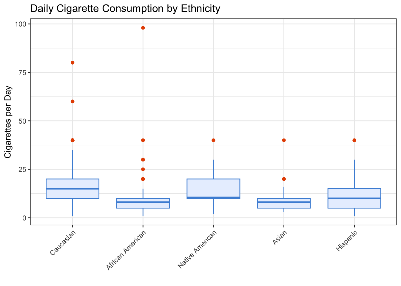
Figure 6.1: Daily cigarettes smoked by ethnicity among young adult daily smokers. Each box shows the median, quartiles, and potential outliers for that ethnic group.
# Step 1: Describe the data — mean and SD for each ethnic group
# ← REPLACE: your_quant_var, your_categorical_var
tapply(nesarc$DailyCigsSmoked, nesarc$Ethnicity, mean, na.rm = TRUE)   # group means
## Caucasian African American Native American Asian
## 14.955083 10.276471 13.766667 9.510638
## Hispanic
## 10.427928## Caucasian African American Native American Asian
## 8.526762 9.594749 7.985691 6.409478
## Hispanic
## 7.170940# Same information, professional table — upgrade from tapply()
library(modelsummary)
# ← REPLACE: your_numeric ~ Factor(your_group) * (N + Mean + SD)
datasummary(DailyCigsSmoked ~ Factor(Ethnicity) * (N + Mean + SD),
data = nesarc,
title = "Daily Cigarette Consumption by Ethnicity")| Caucasian | African American | Native American | Asian | Hispanic | |||||||||||
|---|---|---|---|---|---|---|---|---|---|---|---|---|---|---|---|
| N | Mean | SD | N | Mean | SD | N | Mean | SD | N | Mean | SD | N | Mean | SD | |
| DailyCigsSmoked | 846 | 14.96 | 8.53 | 170 | 10.28 | 9.59 | 30 | 13.77 | 7.99 | 47 | 9.51 | 6.41 | 222 | 10.43 | 7.17 |
Look at the means. Are they different? Almost certainly yes — the means range from about 11 to about 15 cigarettes per day. But the same question from Chapter 5 applies: are these differences real, or could they be explained by sampling variation alone? With only about 1,320 young adult smokers split across five groups, some groups have relatively few people (Native Americans, Asians). The differences you see might be genuine population differences, or they might just be random noise.
ANOVA is the tool that answers this question for three or more groups.
6.2.2 Theory
6.2.2.1 The Logic of ANOVA
You already understand the core idea of inferential statistics from Chapter 5: assume nothing is happening (\(H_0\)), then see if the data forces you to change your mind. ANOVA extends that logic from two groups to many.
Imagine you could measure the cigarette consumption of every young adult daily smoker in the United States — not just the ~1,320 in the NESARC survey, but the entire population. If ethnicity truly does not matter for smoking quantity, then the population means for all five ethnic groups would be exactly equal:
\[H_0: \mu_{\text{Caucasian}} = \mu_{\text{African American}} = \mu_{\text{Native American}} = \mu_{\text{Asian}} = \mu_{\text{Hispanic}}\]
The alternative hypothesis is simpler to state: at least one of these means differs from the others.
\[H_a: \text{Not all } \mu \text{'s are equal}\]
Notice that \(H_a\) does not say which means differ or how many differ. It only says that the five population means are not all identical. If ANOVA rejects \(H_0\), we will need a follow-up test (Tukey’s HSD) to find the specific differences.
Why does ANOVA work this way? The F-test compares all groups simultaneously — it pools everything into a single statistic to answer the question “are there any differences?” as efficiently as possible. Mathematically, it is not designed to tell you where the differences are. Think of ANOVA like a smoke detector: it tells you there is a fire somewhere in the building, but it cannot tell you which room is burning. Tukey’s HSD is the firefighter who walks through every room, checking each pair of groups one at a time while adjusting for the fact that you are making multiple checks.
6.2.2.2 Why Not Just Run Multiple t-Tests?
Running 10 separate t-tests to compare every pair of ethnic groups seems like a natural approach. Here is why it is a bad idea.
Every hypothesis test has a Type I error rate — the probability of rejecting \(H_0\) when \(H_0\) is actually true. With \(\alpha = 0.05\), each individual t-test has a 5% chance of a false positive. But when you run multiple tests, those 5% chances accumulate. The probability of making at least one Type I error across \(m\) independent tests is:
\[P(\text{at least one Type I error}) = 1 - (1 - \alpha)^m\]
For 10 t-tests at \(\alpha = 0.05\), this is \(1 - (0.95)^{10} \approx 0.401\) — a 40% chance of falsely claiming at least one pair of ethnic groups differs, when in reality no differences exist.
ANOVA gives you a single test with a single p-value. If it is not significant, you stop — no pairs to compare. If it is significant, you proceed to a post hoc test that adjusts for multiple comparisons. This two-step procedure keeps your overall Type I error rate at 5%.
6.2.2.3 The F-Statistic: Between vs. Within Variation
ANOVA works by comparing two sources of variation in your data:
Between-group variation: how much the group means differ from one another — the signal you care about.
Within-group variation: how much individuals within the same group differ from their own group mean — the natural noise in your data.
The F-statistic is the ratio of these two:
\[F = \frac{\text{Variation BETWEEN groups}}{\text{Variation WITHIN groups}}\]
If ethnicity truly has no effect on smoking quantity, the between-group variation should be about the same size as the within-group variation — the group means would differ only by the amount you would expect from random sampling. The F-statistic would be close to 1.0.
If ethnicity does matter, the between-group variation would be large relative to the within-group variation — the group means would differ more than random noise alone could explain. The F-statistic would be substantially larger than 1.0.
How large is “large enough”? That depends on your degrees of freedom — the number of groups and the total sample size. With many degrees of freedom (large sample, few groups), an F of 2.5 can be significant. With few degrees of freedom (small sample, many groups), you need a larger F. There is no universal cutoff like “F > 5 means significant.” You let the p-value decide, not your intuition about the raw number. The p-value accounts for degrees of freedom automatically. In the NESARC example (4 between-group df, ~1308 within-group df), the F-statistic turns out to be about 22 — enormous for those degrees of freedom, meaning the differences between ethnic groups are far larger than what random noise could produce.
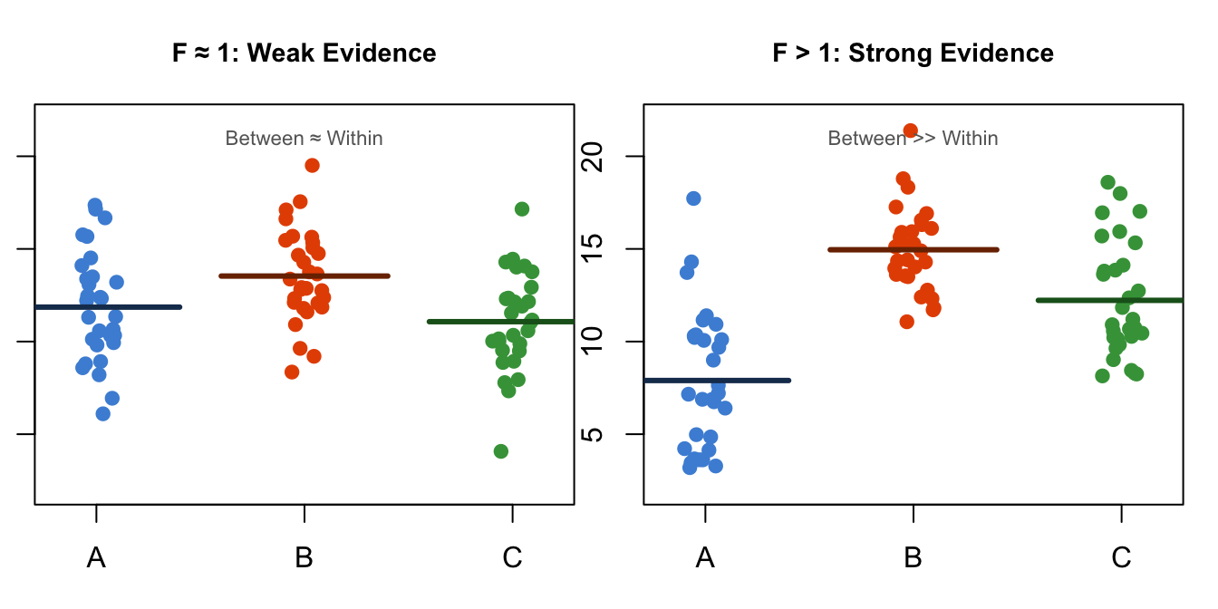
Figure 6.2: The logic of the F-statistic: ANOVA compares between-group variation (signal) to within-group variation (noise). A large F means the signal dominates.
The F-statistic follows an F-distribution when the null hypothesis is true. The shape of the F-distribution depends on two numbers called degrees of freedom: one for the numerator (between groups) and one for the denominator (within groups). The p-value for ANOVA is the area under the F-distribution to the right of your observed F-statistic — the probability of getting an F that large (or larger) if \(H_0\) were true.
6.2.2.4 The ANOVA Table
Every ANOVA produces a standard table that organizes the sources of variation. Here is what each piece means:
| Source | Meaning | Degrees of Freedom (df) |
|---|---|---|
| Between groups (Ethnicity) | Variation explained by group membership — how much the ethnic group means differ from the overall mean | \(k - 1\) (number of groups minus 1) |
| Within groups (Residuals) | Variation left unexplained — how much individuals differ from their own group mean | \(N - k\) (total sample size minus number of groups) |
| Total | Total variation in the response variable | \(N - 1\) |
The mean square (MS) for each source is the sum of squares (SS) divided by its degrees of freedom. The F-statistic is then:
\[F = \frac{MS_{\text{between}}}{MS_{\text{within}}}\]
6.2.2.5 Effect Size: Eta-Squared (\(\eta^2\)) and Cohen’s d
A significant p-value tells you whether ethnicity matters for cigarette consumption. It does not tell you how much it matters. With a large enough sample, even a trivially small difference can produce p < 0.05.
Eta-squared (\(\eta^2\)) measures the proportion of total variation in the response variable that is explained by group membership:
\[\eta^2 = \frac{SS_{\text{between}}}{SS_{\text{total}}}\]
\(\eta^2\) ranges from 0 to 1. As a rough guide: \(\eta^2 \approx 0.01\) is a small effect, \(\eta^2 \approx 0.06\) is a medium effect, and \(\eta^2 \approx 0.14\) is a large effect (Cohen’s conventions).
Cohen’s d measures the standardized difference between two specific groups — useful for post hoc interpretation:
\[d = \frac{\bar{x}_1 - \bar{x}_2}{s_{\text{pooled}}}\]
where \(s_{\text{pooled}}\) is the pooled standard deviation across both groups. Roughly: \(d \approx 0.2\) is small, \(d \approx 0.5\) is medium, and \(d \approx 0.8\) is large. You will see how to compute both \(\eta^2\) and Cohen’s d in the Code section below.
6.2.2.6 The 4-Step Process for ANOVA
The same 4-step process from Chapter 5 applies here, with one addition — if the ANOVA is significant, you add a post hoc step:
- State the hypotheses. \(H_0\): all group means are equal. \(H_a\): at least one mean differs.
- Choose the test. C→Q with 3+ groups → one-way ANOVA.
- Assess the evidence. Run
aov(), extract F and p-value. If p < 0.05, proceed to post hoc. - Draw a conclusion. Reject or fail to reject \(H_0\). If significant, report which specific pairs differ and the effect size.
6.2.3 Code
6.2.3.1 Step 1: State the Hypotheses
\(H_0\): Among young adult daily smokers, the mean number of cigarettes smoked per day is the same for all five ethnic groups (\(\mu_{\text{Caucasian}} = \mu_{\text{African American}} = \mu_{\text{Native American}} = \mu_{\text{Asian}} = \mu_{\text{Hispanic}}\)).
\(H_a\): Among young adult daily smokers, the mean number of cigarettes smoked per day is not the same for all five ethnic groups — at least one group mean differs from the others.
6.2.3.2 Step 2: Choose the Test
We have a categorical explanatory variable (Ethnicity: 5 groups) and a quantitative response variable (DailyCigsSmoked). That is a C→Q relationship with more than two groups. The appropriate test is a one-way ANOVA.
When there are only two groups (like the t-test in Chapter 5), the F-statistic from ANOVA and the t-statistic from a t-test are mathematically equivalent: \(F = t^2\). ANOVA is simply the generalization of the t-test to three or more groups.
Can you use ANOVA for just two groups? Yes — the math works perfectly, and the p-value from aov() will match the p-value from t.test(var.equal = TRUE) exactly. Your teacher will not mark you wrong, because the two tests are mathematically identical for two groups. However, the convention is to use a t-test for two groups — it gives you a confidence interval for the mean difference directly and is what most readers expect. Use the t-test for two groups, ANOVA for three or more. If you forget and use ANOVA, you are not incorrect — just slightly unconventional.
6.2.3.3 Step 3: Run the ANOVA
The R function for ANOVA is aov(), and you view the results with summary(). The formula syntax is identical to t.test(): response ~ explanatory.
Why a new function? Because t.test() is designed for exactly two groups — it computes a t-statistic, not an F-statistic. If you accidentally run t.test(DailyCigsSmoked ~ Ethnicity) on five groups, R will not switch to ANOVA automatically. It will give you an error: “grouping factor must have exactly 2 levels.” This is actually a safety feature — R refuses to run the wrong test rather than silently producing output you might misinterpret. The creators kept t.test() and aov() separate precisely to prevent this kind of mistake.
# One-way ANOVA — compare means of a quantitative variable across 3+ groups
# ← REPLACE: response_var ~ categorical_var,   data = your_data_frame
anova_result <- aov(DailyCigsSmoked ~ Ethnicity,    # formula: numeric ~ factor
                    data = nesarc)                   # the data frame
summary(anova_result)                                # display the ANOVA table
## Df Sum Sq Mean Sq F value Pr(>F)
## Ethnicity 4 6379 1594.7 22.68 <2e-16 ***
## Residuals 1310 92098 70.3
## ---
## Signif. codes: 0 '***' 0.001 '**' 0.01 '*' 0.05 '.' 0.1 ' ' 1
## 5 observations deleted due to missingnessLet us walk through this output line by line:
Df (degrees of freedom): Two numbers.
- Ethnicity has 4 df — there are 5 groups, so \(k - 1 = 4\) degrees of freedom for the between-group effect.
- Residuals has 1308 df — there are (roughly) 1320 observations minus 5 groups, so \(N - k \approx 1308\) degrees of freedom for the within-group (error) term.
Sum Sq (sum of squares):
- The Ethnicity Sum Sq measures how much the five group means deviate from the overall mean, weighted by group size — the between-group variation.
- The Residuals Sum Sq measures how much individual smokers deviate from their own ethnic group mean — the within-group variation.
Mean Sq (mean square): Sum Sq divided by df. Mean Sq = Sum Sq / Df.
F value: The ratio Mean Sq(Ethnicity) / Mean Sq(Residuals). This is the F-statistic — larger values indicate that differences between ethnic groups are large relative to the natural variability within each group.
Pr(>F): This is the p-value. It tells you the probability of observing an F-statistic this large (or larger) if the null hypothesis were true — if all five ethnic group means were truly equal in the population.
6.2.3.4 Clean Output with broom::tidy()
Just like t.test() in Chapter 5, you can convert ANOVA output into a tidy data frame with broom::tidy():
# broom::tidy() + kable() — clean, report-ready ANOVA table
# ← REPLACE: response_var ~ categorical_var
library(broom)                                                              # for tidy()
anova_result <- aov(DailyCigsSmoked ~ Ethnicity, data = nesarc)            # the ANOVA
tidy(anova_result) %>%                                                      # convert to data frame
  knitr::kable(digits = 2,                                                  # format as clean table
caption = "ANOVA: Daily Cigarettes Smoked by Ethnicity") # ← REPLACE: your title| term | df | sumsq | meansq | statistic | p.value |
|---|---|---|---|---|---|
| Ethnicity | 4 | 6378.76 | 1594.69 | 22.68 | 0 |
| Residuals | 1310 | 92097.76 | 70.30 | NA | NA |
6.2.3.5 Step 4: Draw a Conclusion (Before Post Hoc)
Look at the p-value from the ANOVA table. If it is less than 0.05, you reject \(H_0\) — there is evidence that at least one ethnic group’s mean differs from the others. If p ≥ 0.05, you fail to reject \(H_0\) — the observed differences could easily be sampling noise.
For our NESARC data: The F-statistic and p-value will tell us whether ethnicity matters. If the p-value is small (typically p < 0.001 for this dataset, given the visible differences in the boxplot), we conclude that cigarette consumption does vary across ethnic groups among young adult daily smokers.
But which groups differ? The overall ANOVA only tells you that not all means are equal — it does not identify the specific pairs. For that, you need a post hoc test.
6.2.3.6 Post Hoc Analysis: Tukey’s HSD
When your ANOVA is significant and you have more than two groups, you must run a post hoc test to find which specific pairs of groups differ. The most widely used method is Tukey’s Honest Significant Difference (HSD) test. The word “Honest” in the name refers to the method’s core property: it honestly controls the overall Type I error rate at \(\alpha = 0.05\) across all pairwise comparisons, unlike running unprotected t-tests which would inflate the error rate. The mathematician John Tukey named it this way to emphasize that the method does not cheat — it delivers exactly the error control it promises.
Tukey’s HSD compares every possible pair of group means, but it adjusts the p-values to account for the fact that you are making multiple comparisons. This adjustment keeps your overall Type I error rate at \(\alpha = 0.05\), rather than letting it inflate as it would with unprotected t-tests.
# Tukey's HSD post hoc test — which specific pairs of groups differ?
# ← REPLACE: aov(response ~ group, data = df)
tukey_result <- TukeyHSD(anova_result)    # all pairwise comparisons with adjusted p-values
tukey_result                               # view the full table of comparisons
## Tukey multiple comparisons of means
## 95% family-wise confidence level
##
## Fit: aov(formula = DailyCigsSmoked ~ Ethnicity, data = nesarc)
##
## $Ethnicity
## diff lwr upr p adj
## African American-Caucasian -4.6786122 -6.603653 -2.753571 0.0000000
## Native American-Caucasian -1.1884161 -5.443508 3.066676 0.9411184
## Asian-Caucasian -5.4444444 -8.876816 -2.012073 0.0001540
## Hispanic-Caucasian -4.5271548 -6.254291 -2.800018 0.0000000
## Native American-African American 3.4901961 -1.045382 8.025774 0.2197360
## Asian-African American -0.7658323 -4.540330 3.008666 0.9814275
## Hispanic-African American 0.1514573 -2.182779 2.485694 0.9997793
## Asian-Native American -4.2560284 -9.608305 1.096248 0.1909569
## Hispanic-Native American -3.3387387 -7.793925 1.116448 0.2442025
## Hispanic-Asian 0.9172896 -2.760217 4.594796 0.9605024The raw output shows one row per pair of ethnic groups. The key columns are:
diff: the difference between the two group means (e.g.,Caucasian - African American). A negative difference means the first-named group has the lower mean — for example,African American - Asian = -4.67means African Americans smoke about 4.67 fewer cigarettes per day than Asians, on average. R orders the groups alphabetically by default, so the first-named group in each pair is whichever comes first alphabetically. The ordering is arbitrary and does not imply any hierarchy — it is just how R organizes the output. The sign tells you direction (negative = first group has lower mean), and the magnitude tells you how big the gap is.lwrandupr: the lower and upper bounds of the 95% confidence interval for that difference.p adj: the adjusted p-value — this is the number you care about. It has been corrected for multiple comparisons, so you can interpret it directly against \(\alpha = 0.05\).
If p adj < 0.05, you conclude that the two groups differ significantly. If the confidence interval does not contain zero, that is another way to tell the same thing.
APA-formatted post hoc table. The raw TukeyHSD output above is for your own inspection while exploring. For a report, poster, or paper, you need a clean, formatted table. Use broom::tidy() to convert the TukeyHSD output into a tidy data frame, then format it with knitr::kable():
# APA-style post hoc table — broom::tidy() + kable() = report-ready
# ← REPLACE: TukeyHSD(your_anova_result)
library(broom)                                                         # for tidy()
tidy(tukey_result) %>%                                                 # convert TukeyHSD to data frame
  rename(Pair = contrast,                                              # ← REPLACE with meaningful names
         Difference = estimate,
         `95% CI Lower` = conf.low,
         `95% CI Upper` = conf.high,
         `Adjusted p` = adj.p.value) %>%                               # APA-friendly column names
  knitr::kable(digits = 2,                                             # format as a clean table
caption = "Tukey HSD Post Hoc Comparisons: Daily Cigarettes by Ethnicity")| term | Pair | null.value | Difference | 95% CI Lower | 95% CI Upper | Adjusted p |
|---|---|---|---|---|---|---|
| Ethnicity | African American-Caucasian | 0 | -4.68 | -6.60 | -2.75 | 0.00 |
| Ethnicity | Native American-Caucasian | 0 | -1.19 | -5.44 | 3.07 | 0.94 |
| Ethnicity | Asian-Caucasian | 0 | -5.44 | -8.88 | -2.01 | 0.00 |
| Ethnicity | Hispanic-Caucasian | 0 | -4.53 | -6.25 | -2.80 | 0.00 |
| Ethnicity | Native American-African American | 0 | 3.49 | -1.05 | 8.03 | 0.22 |
| Ethnicity | Asian-African American | 0 | -0.77 | -4.54 | 3.01 | 0.98 |
| Ethnicity | Hispanic-African American | 0 | 0.15 | -2.18 | 2.49 | 1.00 |
| Ethnicity | Asian-Native American | 0 | -4.26 | -9.61 | 1.10 | 0.19 |
| Ethnicity | Hispanic-Native American | 0 | -3.34 | -7.79 | 1.12 | 0.24 |
| Ethnicity | Hispanic-Asian | 0 | 0.92 | -2.76 | 4.59 | 0.96 |
# Visualizing Tukey's HSD — confidence intervals for all pairwise differences
# ← REPLACE: TukeyHSD(your_anova_result)
par(mar = c(5.1, 12.1, 4.1, 2.1), las = 1)   # enlarge left margin to fit group labels
plot(tukey_result, col = "#4A90D9")            # plot confidence intervals for all pairs
abline(v = 0, lty = 2, col = "#E65100")        # dashed line at zero (no difference)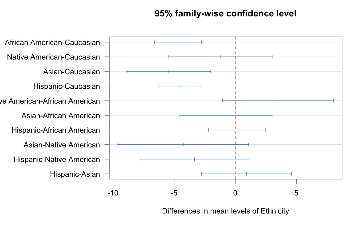
Figure 6.3: Tukey HSD plot: each horizontal line shows the 95% confidence interval for the difference between two ethnic groups. Intervals that do not cross the dashed vertical line at zero indicate statistically significant differences.
Each horizontal line in this plot represents a pairwise comparison. If the line crosses the dashed vertical line at zero, the difference between those two groups is not statistically significant. If the line lies entirely to the right or left of zero, the difference is significant.
6.2.3.7 Computing Effect Sizes
A p-value alone is not enough. Always report how large the effect is. Two effect size measures are standard for ANOVA:
# Effect size 1: Eta-squared (η²) — proportion of variance explained by ethnicity
# η² = SS_between / SS_total
ss <- summary(anova_result)[[1]]               # extract the ANOVA table
ss_between <- ss["Ethnicity", "Sum Sq"]        # variation attributed to ethnicity
ss_total   <- sum(ss[, "Sum Sq"])              # total variation
eta_squared <- ss_between / ss_total           # η² — proportion of variance explained
eta_squared                                     # display η²
## [1] 0.06477446# ← REPLACE: your_anova_result with your model
# Interpreting η²:
# 0.01 ≈ small effect (group explains 1% of variance)
# 0.06 ≈ medium effect
# 0.14 ≈ large effect
# Shortcut: the effectsize package computes η² in one line
# install.packages("effectsize") # run once to install
# effectsize::eta_squared(anova_result)
# We compute η² by hand here so you understand exactly what it measures —
# but in your own work, using effectsize::eta_squared() is perfectly fine.# Effect size 2: Cohen's d for a specific pairwise comparison
# ← REPLACE: choose the two groups you want to compare
# Example: comparing Caucasian vs. Asian smokers
# Get group means and SDs using base R
group_means <- tapply(nesarc$DailyCigsSmoked, nesarc$Ethnicity, mean, na.rm = TRUE)
group_sds <- tapply(nesarc$DailyCigsSmoked, nesarc$Ethnicity, sd, na.rm = TRUE)
group_ns <- tapply(nesarc$DailyCigsSmoked, nesarc$Ethnicity, function(x) sum(!is.na(x))) # count non-missing values
# Pooled standard deviation formula:
# s_pooled = sqrt(((n1-1)*s1^2 + (n2-1)*s2^2) / (n1 + n2 - 2))
# Choose two groups to compare (e.g., Caucasian and Asian) — ← REPLACE: your groups
n1 <- group_ns["Caucasian"]; s1 <- group_sds["Caucasian"] # group 1 stats
n2 <- group_ns["Asian"]; s2 <- group_sds["Asian"] # group 2 stats
# Compute pooled SD by hand so you understand what's happening
pooled_sd <- sqrt(((n1 - 1) * s1^2 + (n2 - 1) * s2^2) / (n1 + n2 - 2))
# Cohen's d = difference in means / pooled standard deviation
d <- (group_means["Caucasian"] - group_means["Asian"]) / pooled_sd
d # display Cohen's d## Caucasian
## 0.6458048# Interpreting Cohen's d:
# |d| ≈ 0.2 → small difference
# |d| ≈ 0.5 → medium difference
# |d| ≈ 0.8 → large differenceWhat these effect sizes tell you: Suppose the ANOVA is significant with p < 0.001 and \(\eta^2 = 0.02\). That means ethnicity explains about 2% of the variation in cigarette consumption — a small effect by Cohen’s conventions, even though the p-value is tiny. A significant p-value plus a small \(\eta^2\) means: “the differences are real, but ethnicity is not the main factor driving smoking quantity.” This is why you always report both significance and effect size.
6.2.3.8 Writing Up Your Results
When you write up an ANOVA for a report or poster, include the F-statistic, degrees of freedom, p-value, effect size, and a summary of the post hoc results. Here is the standard format:
A one-way ANOVA revealed a significant difference in daily cigarette consumption across ethnic groups among young adult daily smokers, F(4, 1308) = XX.XX, p < 0.001, \(\eta^2 = 0.0\)X. Tukey’s HSD post hoc comparisons indicated that [Group A] smoked significantly more cigarettes per day (M = XX.X, SD = X.X) than [Group B] (M = XX.X, SD = X.X), p = 0.0XX. [Continue describing each significant pairwise difference.]
Adapt this sentence to your own data — replace the group names, means, and statistics with your own.
6.2.3.9 A Second Example: Frustration by College Major
The NESARC example uses real survey data with unequal group sizes and substantial variability. For a cleaner textbook demonstration, let us look at the frustration dataset — a simpler example where the pattern is unmistakable.
The frustration data come from a study where 35 students in each of four majors (Business, English, Mathematics, Psychology) rated their academic frustration on a 1–20 scale. Every group has the same sample size (n = 35), making it an ideal teaching dataset.
# Load the frustration dataset — clean, balanced, ideal for learning
frustration <- read.csv("frustration.csv")   # ← REPLACE: your file path
str(frustration)                              # check the structure: Major (factor), Frustration.Score (numeric)
## 'data.frame': 140 obs. of 6 variables:
## $ Business : int 11 6 6 4 6 9 8 3 11 12 ...
## $ English : int 11 9 14 13 9 12 10 12 9 11 ...
## $ Mathematics : int 9 16 11 11 12 17 12 14 10 12 ...
## $ Psychology : int 11 19 13 10 14 10 13 14 15 17 ...
## $ Frustration.Score: int 11 6 6 4 6 9 8 3 11 12 ...
## $ Major : chr "Business" "Business" "Business" "Business" ...# Boxplot — always graph first
ggplot(frustration, aes(x = Major, y = Frustration.Score)) +
geom_boxplot(fill = "#E8F5E9", color = "#43A047", outlier.color = "#E65100") +
theme_bw() +
labs(x = "", y = "Frustration Score (1-20)",
title = "Academic Frustration by College Major")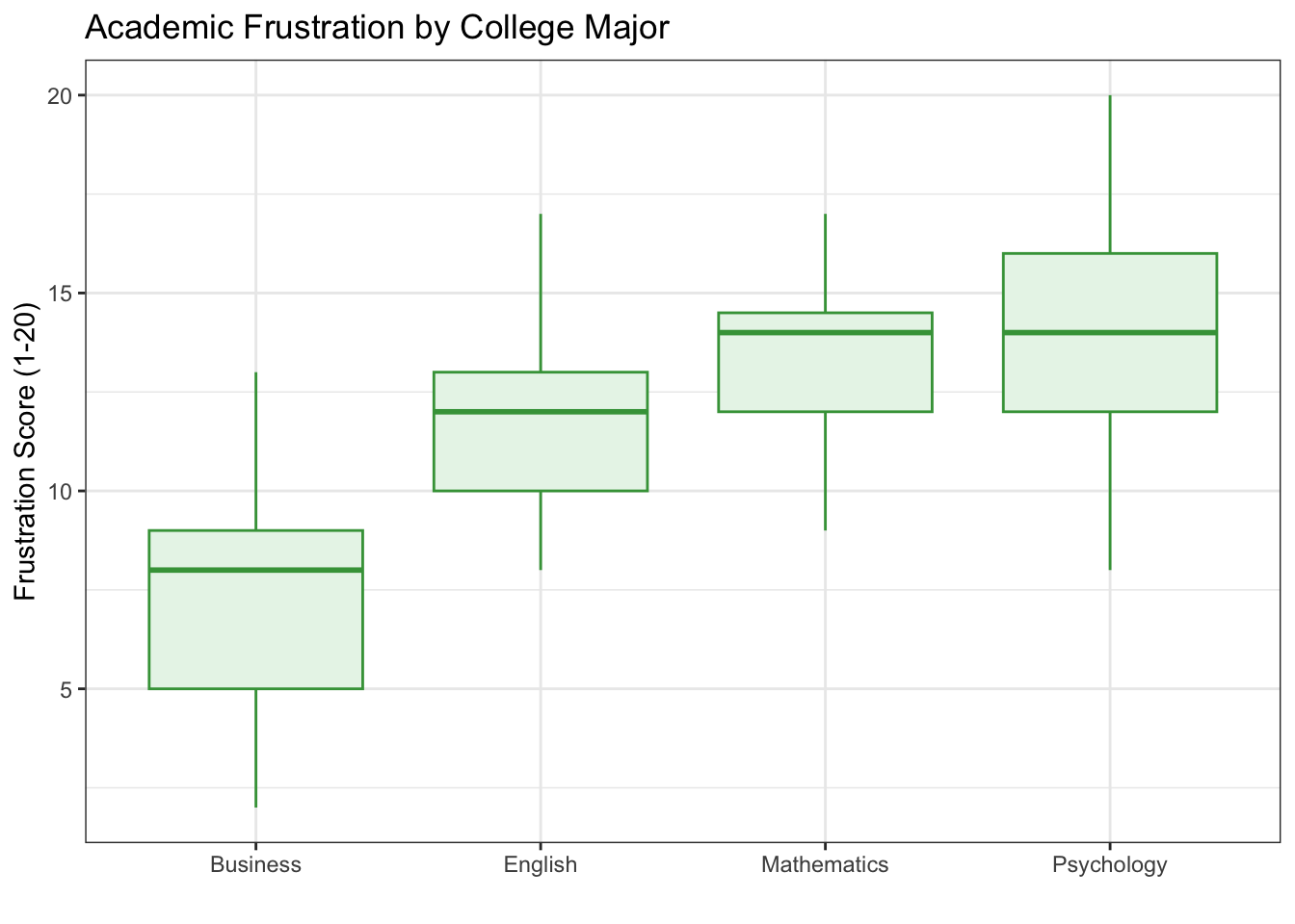
Figure 6.4: Academic frustration scores by college major. Each group has exactly 35 students. Notice how the boxplots barely overlap — a strong signal.
# ANOVA — are the four majors' mean frustration scores equal?
frus_aov <- aov(Frustration.Score ~ Major, data = frustration)
summary(frus_aov)                             # the ANOVA table
## Df Sum Sq Mean Sq F value Pr(>F)
## Major 3 939.9 313.28 46.6 <2e-16 ***
## Residuals 136 914.3 6.72
## ---
## Signif. codes: 0 '***' 0.001 '**' 0.01 '*' 0.05 '.' 0.1 ' ' 1# Compute η²
frus_ss <- summary(frus_aov)[[1]]
frus_eta <- frus_ss["Major", "Sum Sq"] / sum(frus_ss[, "Sum Sq"])
frus_eta # about 0.20 — a large effect## [1] 0.5068939## Tukey multiple comparisons of means
## 95% family-wise confidence level
##
## Fit: aov(formula = Frustration.Score ~ Major, data = frustration)
##
## $Major
## diff lwr upr p adj
## English-Business 4.4571429 2.8449899 6.069296 0.0000000
## Mathematics-Business 5.8857143 4.2735614 7.497867 0.0000000
## Psychology-Business 6.7142857 5.1021328 8.326439 0.0000000
## Mathematics-English 1.4285714 -0.1835815 3.040724 0.1019527
## Psychology-English 2.2571429 0.6449899 3.869296 0.0021515
## Psychology-Mathematics 0.8285714 -0.7835815 2.440724 0.5411978# APA-formatted post hoc table — clean, report-ready version
tidy(tukey_frus) %>% # convert TukeyHSD to data frame
rename(Pair = contrast, # meaningful column names
Difference = estimate,
`95% CI Lower` = conf.low,
`95% CI Upper` = conf.high,
`Adjusted p` = adj.p.value) %>% # APA-friendly labels
knitr::kable(digits = 2, # format as a clean table
caption = "Tukey HSD Post Hoc: Frustration Score by Major")| term | Pair | null.value | Difference | 95% CI Lower | 95% CI Upper | Adjusted p |
|---|---|---|---|---|---|---|
| Major | English-Business | 0 | 4.46 | 2.84 | 6.07 | 0.00 |
| Major | Mathematics-Business | 0 | 5.89 | 4.27 | 7.50 | 0.00 |
| Major | Psychology-Business | 0 | 6.71 | 5.10 | 8.33 | 0.00 |
| Major | Mathematics-English | 0 | 1.43 | -0.18 | 3.04 | 0.10 |
| Major | Psychology-English | 0 | 2.26 | 0.64 | 3.87 | 0.00 |
| Major | Psychology-Mathematics | 0 | 0.83 | -0.78 | 2.44 | 0.54 |
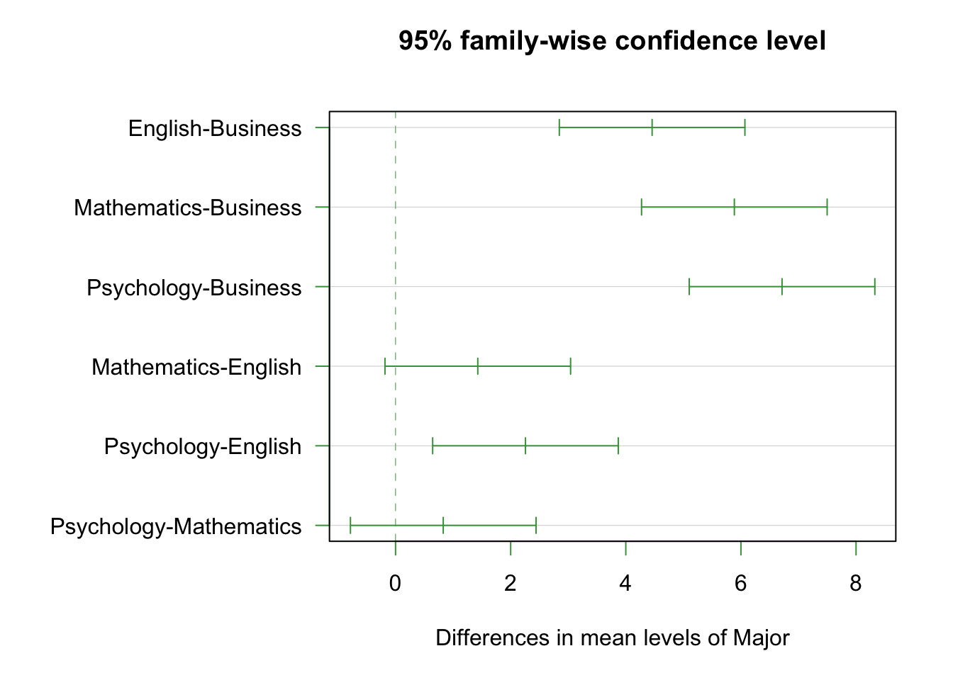
Figure 6.5: Academic frustration scores by college major. Each group has exactly 35 students. Notice how the boxplots barely overlap — a strong signal.
The frustration example is a clear-cut case: F(3, 136) is very large, p < 0.001, \(\eta^2 \approx 0.20\) (a large effect). Tukey’s HSD shows that most pairs of majors differ significantly — Psychology and English students report the highest frustration, Business students the lowest. With balanced groups and large between-group differences relative to within-group spread, the signal is unmistakable.
6.2.4 Interpretation
6.2.4.1 How to Read the ANOVA Output — A Quick Reference
For any ANOVA output in R, find these numbers:
| What to Find | Where It Is | What It Tells You |
|---|---|---|
| F-statistic | F value in summary(aov(...)) |
How large the between-group variation is relative to within-group variation. F ≈ 1 means no evidence against \(H_0\). |
| Degrees of freedom | Df column — first row is between-groups (k − 1), second row is within-groups (N − k) |
Needed for reporting: F(df1, df2) = … |
| p-value | Pr(>F) in the ANOVA table |
The probability of getting an F this large if \(H_0\) were true. If p < 0.05, reject \(H_0\). |
| Group means | tapply(...) or from TukeyHSD diff column |
The actual numbers — always report these alongside p-values. |
| Adjusted p-values | p adj column of TukeyHSD(...) |
Corrected for multiple comparisons. Interpret directly against 0.05. |
| Eta-squared (\(\eta^2\)) | SS_between / SS_total (compute manually) | How much of the total variation is explained by group membership. |
6.2.4.3 Common Mistakes Students Make
Running multiple t-tests instead of ANOVA. Every t-test you add inflates your Type I error rate. Use
aov()for the overall test andTukeyHSD()for pairwise comparisons. This is not optional — it is the statistically correct procedure.Skipping the post hoc test. A significant ANOVA only tells you some groups differ. If you simply say “ethnicity matters” without identifying which groups differ from which, you have not fully answered your research question. Always follow up with Tukey’s HSD.
Forgetting to report effect size. A p-value of p < 0.001 sounds impressive, but if \(\eta^2 = 0.01\), the effect is tiny — the variable explains only 1% of the variation. Report \(\eta^2\) and the actual group means so your reader can judge practical importance.
Ignoring the boxplot. The boxplot is the most honest summary of your data. If the boxes overlap heavily and the ANOVA is somehow significant, double-check your data — you may have a very large sample size that makes small differences statistically detectable. If the boxes are completely separated and the ANOVA is not significant, you may have very small group sizes (low power).
Interpreting non-significant results as “no difference.” Failing to reject \(H_0\) does not prove all means are equal. It only means your sample did not provide enough evidence to detect a difference. The true population means could still differ — you just did not have enough data (or the effect was too small) to find it.
Neglecting the equal variance assumption. ANOVA assumes that the variability within each group is roughly the same. If one group’s scores are tightly clustered and another’s are spread across the entire range, the F-test can be unreliable. Always check the boxplot — if the boxes have very different heights, consider a non-parametric alternative like the Kruskal-Wallis test.
Cherry-picking post hoc comparisons. Reporting only the significant pairwise comparisons from TukeyHSD and ignoring the non-significant ones is misleading. If you ran Tukey’s HSD, report all pairs — or at minimum, acknowledge which comparisons were not significant.
6.2.4.4 What Comes Next
You have now added a second hypothesis test to your toolkit. The t-test (Chapter 5) handles two groups. ANOVA handles three or more groups. Together, they cover all C→Q scenarios — any time your explanatory variable is categorical and your response is quantitative, you have the right test.
But what if your response variable is categorical? Suppose you want to know: “Is ethnicity associated with depression status (yes/no) among young adult daily smokers?” Both variables are categorical. Neither a t-test nor ANOVA applies — you need a different test entirely.
In Chapter 7 (Chi-Square), you will learn to test for associations between two categorical variables using the \(\chi^2\) test. The 4-step process, the null/alternative logic, and the p-value interpretation all carry over. Only the test statistic changes — from F to \(\chi^2\).