Chapter 5 Hypothesis Testing

5.1 TL;DR: Hypothesis Testing

Inferential statistics moves from describing data to testing whether patterns are real or just sampling noise.
A hypothesis test asks: “If there were truly no effect, how likely is it that I would see data like mine?” That probability is the p-value.
The null hypothesis ($H_0$) says nothing is happening (no difference, no relationship). The alternative hypothesis ($H_a$) says something is happening.
If p < 0.05, reject $H_0$ — the evidence is strong enough to conclude a real effect exists. If p ≥ 0.05, fail to reject $H_0$ — the evidence is too weak.
The 4-step process is the same for every test in this book: (1) state hypotheses, (2) choose the test, (3) assess the evidence (get the p-value), (4) draw a conclusion.
The test you choose depends on your variable types: C→Q uses t-test or ANOVA, C→C uses Chi-Square, Q→Q uses correlation or regression.

# Load dplyr for filter() and %>%
library(dplyr)

# Load the NESARC survey — ← REPLACE: your file path
NESARC <- read.csv("NESARC.csv")

# Filter to young adult daily smokers — ← REPLACE: your filter logic
nesarc <- NESARC %>%
  filter(
    S3AQ1A == 1,         # smoked 100+ cigarettes in lifetime
    CHECK321 == 1,       # valid nicotine dependence data
    S3AQ3B1 == 1,        # smoked in the past 12 months
    AGE <= 25             # young adults only
  )

# Recode 99 as missing — 99 means "Unknown" in the NESARC code book
nesarc$S3AQ3C1[nesarc$S3AQ3C1 == 99] <- NA    # ← REPLACE: your NA codes

# Label the categorical variable — ← REPLACE: your variable and labels
nesarc$Depression <- factor(nesarc$MAJORDEPLIFE,
  labels = c("No Depression", "Yes Depression"))

# Independent samples t-test — ← REPLACE: quant_var ~ cat_var,   data = your_df
t.test(S3AQ3C1 ~ Depression, data = nesarc, var.equal = TRUE)

## 
##  Two Sample t-test
## 
## data:  S3AQ3C1 by Depression
## t = -1.3692, df = 1313, p-value = 0.1712
## alternative hypothesis: true difference in means between group No Depression and group Yes Depression is not equal to 0
## 95 percent confidence interval:
##  -1.7938413  0.3191162
## sample estimates:
##  mean in group No Depression mean in group Yes Depression 
##                     13.16632                     13.90368

# Clean APA-style results table — tidy() + kable() = report-ready table
library(broom)                                                        # for tidy()
test <- t.test(S3AQ3C1 ~ Depression, data = nesarc, var.equal = TRUE) # run the test
tidy(test) %>%                                                        # convert to data frame
  select(estimate1, estimate2, statistic, p.value, parameter,         # keep key columns
         conf.low, conf.high) %>%
  knitr::kable(digits = 2,                                            # format as a clean table
               caption = "Independent Samples t-test Results")        # ← REPLACE: your title

Table 5.1: Independent Samples t-test Results
estimate1	estimate2	statistic	p.value	parameter	conf.low	conf.high
13.17	13.9	-1.37	0.17	1313	-1.79	0.32

Key interpretation: The NESARC t-test gives p = 0.35 — far above 0.05 — so we fail to reject $H_0$. The observed difference of about 0.4 cigarettes per day is easily explained by sampling variation. There is not enough evidence to conclude depression is associated with smoking quantity.

5.2 Deep Dive: Hypothesis Testing

5.2.1 Motivating Example

Chapters 1 through 4 gave you the tools to describe data — to summarize one variable, to graph the relationship between two, to handle messy data, and to spot patterns. That was all descriptive statistics.

Now it is time to move from description to decision. The question is no longer just “what does my data look like?” but “does my data provide enough evidence to conclude something about the larger world?”

Let us start with a concrete example. Suppose your research question is:

Do young adult daily smokers with depression smoke more cigarettes per day than those without depression?

You have the NESARC dataset — a representative survey of over 43,000 U.S. adults. You subset it to young adults (18–25) who smoke daily (the nesarc data frame you built in Chapter 3). You then calculate the mean number of cigarettes smoked per day for each group.

# Load the packages you need for this chapter
library(ggplot2)      # for all graphing
library(dplyr)        # for filter(), rename(), select(), %>%
library(modelsummary) # for professional summary tables

# Load the NESARC survey (43,093 adults) — ← REPLACE: your file path
NESARC <- read.csv("NESARC.csv")

# Build the subset we use throughout the book:
# young adult (<= 25) daily smokers with valid nicotine data
# ← REPLACE: adapt filter, rename, factor labels to YOUR dataset
nesarc <- NESARC %>%
  filter(
    S3AQ1A == 1,         # smoked 100+ cigarettes in lifetime
    S3AQ3B1 == 1,        # smoked in the past 12 months
    CHECK321 == 1,       # valid nicotine dependence data
    AGE <= 25             # young adults only
  ) %>%
  rename(
    Ethnicity          = ETHRACE2A,     # ← REPLACE: rename to meaningful names
    Age                = AGE,           # age in years
    MajorDepression    = MAJORDEPLIFE,  # lifetime depression diagnosis
    TobaccoDependence  = TAB12MDX,      # tobacco dependence, past 12 months
    DailyCigsSmoked    = S3AQ3C1,       # cigarettes per day (99 = missing)
    Sex                = SEX            # sex (1=Female, 2=Male)
  ) %>%
  select(Ethnicity, Age, MajorDepression, TobaccoDependence, DailyCigsSmoked, Sex)

# Code 99 as missing — 99 means "Unknown" in the NESARC code book
nesarc$DailyCigsSmoked[nesarc$DailyCigsSmoked == 99] <- NA    # ← REPLACE: your NA codes

# Convert numeric codes into readable labels (factors)
nesarc$MajorDepression <- factor(nesarc$MajorDepression,
  labels = c("No Depression", "Yes Depression"))               # ← REPLACE: your labels
nesarc$TobaccoDependence <- factor(nesarc$TobaccoDependence,
  labels = c("No Dependence", "Nicotine Dependence"))          # ← REPLACE: your labels
nesarc$Sex <- factor(nesarc$Sex,
  labels = c("Female", "Male"))                                # ← REPLACE: your labels

# Step 1: Describe the data — mean and SD for each group
# ← REPLACE: your_quant_var ~ your_categorical_var
tapply(nesarc$DailyCigsSmoked, nesarc$MajorDepression, mean, na.rm = TRUE)   # group means

##  No Depression Yes Depression 
##       13.16632       13.90368

tapply(nesarc$DailyCigsSmoked, nesarc$MajorDepression, sd, na.rm = TRUE)     # group SDs

##  No Depression Yes Depression 
##       8.460312       9.162474

# Same information, professional table — upgrade from tapply()
library(modelsummary)
# ← REPLACE: your_numeric ~ Factor(your_group) * (N + Mean + SD)
datasummary(DailyCigsSmoked ~ Factor(MajorDepression) * (N + Mean + SD),
            data = nesarc)

	No Depression			Yes Depression
	N	Mean	SD	N	Mean	SD
DailyCigsSmoked	962	13.17	8.46	353	13.90	9.16

Young adult daily smokers with depression smoke about 13.7 cigarettes per day, on average. Those without depression smoke about 13.2 per day. That is a difference of about half a cigarette per day.

Here is the critical question: is this difference real, or is it just random chance?

Think about what “random chance” means here. The NESARC survey sampled about 43,000 people out of a U.S. adult population of over 200 million. Even if depression and smoking are completely unrelated in the full population, a random sample of 1,320 young smokers might — just by luck — have one group smoke a bit more than the other. The difference you see could be nothing more than sampling noise.

That is the central problem Statistical inference solves. In this chapter, you will learn how to answer the question “Is this pattern real?” using the most fundamental tool in inferential statistics: the hypothesis test.

5.2.2 Theory

5.2.2.1 The Logic of Hypothesis Testing

Hypothesis testing is built on a simple idea that you already use in everyday life: assume nothing is going on, then see if the evidence forces you to change your mind.

Think of a courtroom. The defendant is presumed innocent until proven guilty. The prosecution must provide enough evidence to convince the jury beyond a reasonable doubt. If the evidence is weak, the defendant walks free — not because we proved innocence, but because we failed to prove guilt.

Statistical hypothesis testing works the same way:

Assume the “innocent” explanation: there is no real difference, no real relationship. The pattern you see is just sampling noise. This is called the null hypothesis ($H_0$).
Gather evidence: collect data from a sample and calculate a test statistic — a number that summarizes the pattern in your data (like the difference between two group means).
Ask: how surprising is this evidence? If the null hypothesis were true, how often would random sampling produce a difference at least as large as what we observed? This probability is the p-value.
Make a decision: if the p-value is small enough, the evidence is strong enough to reject the null hypothesis. We conclude there is a real effect. If the p-value is not small enough, we “fail to reject” the null — the evidence is too weak to reach a firm conclusion.

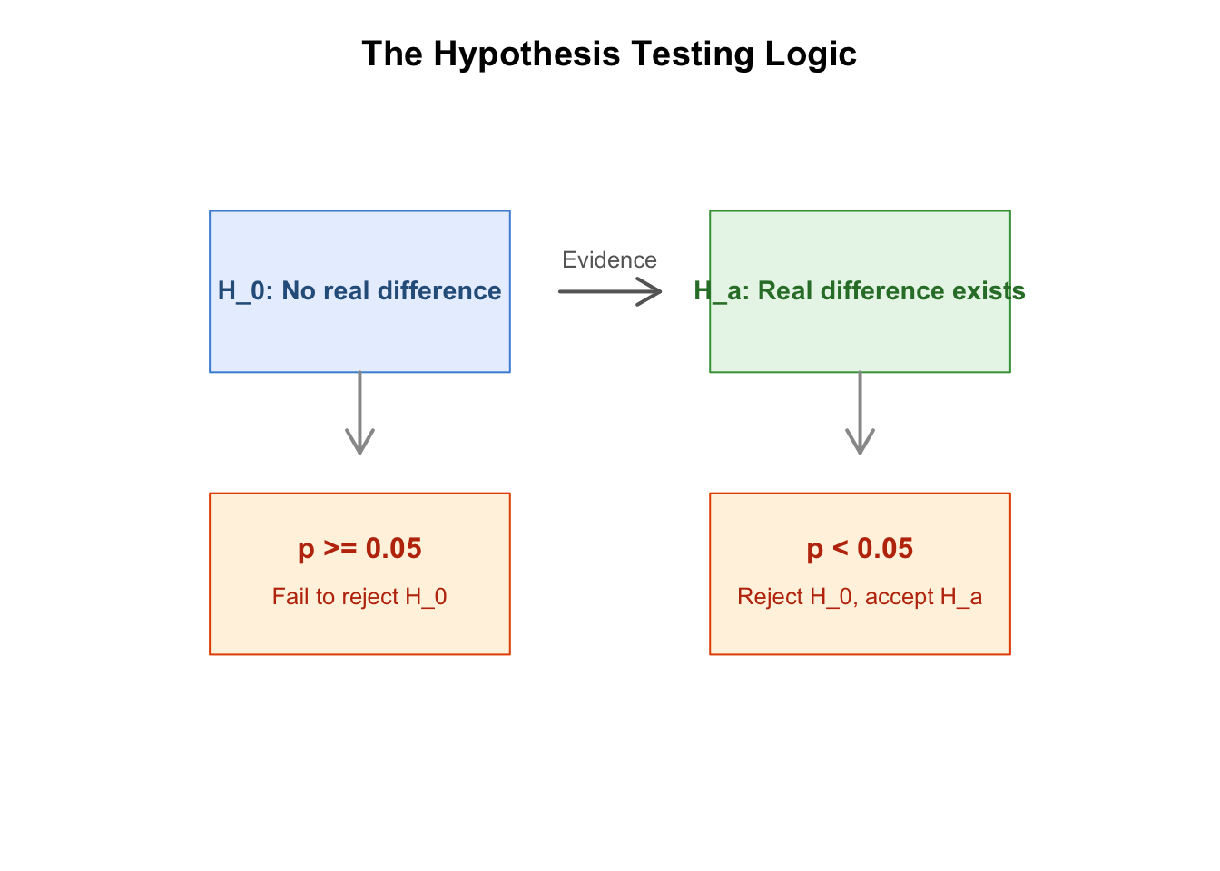
Figure 5.1: The logic of hypothesis testing: assume the null, assess evidence, make a decision.

This logic applies to every statistical test you will learn in this book — ANOVA, Chi-Square, correlation, regression. The test itself changes, but the reasoning is always the same.

5.2.2.2 The Null Hypothesis ($H_0$) and Alternative Hypothesis ($H_a$)

For our smoking and depression example:

$H_0$ (null): In the population of young adult daily smokers, the mean number of cigarettes smoked per day is the same for those with and without depression. Formally: $\mu_{\text{depression}} = \mu_{\text{no depression}}$, or $\mu_{\text{depression}} - \mu_{\text{no depression}} = 0$.
$H_a$ (alternative): In the population, the mean number of cigarettes smoked differs between those with and without depression. Formally: $\mu_{\text{depression}} \neq \mu_{\text{no depression}}$, or $\mu_{\text{depression}} - \mu_{\text{no depression}} \neq 0$.

Notice the language: the null hypothesis always contains an equals sign ($=$, $\le$, or $\ge$). It is the “nothing is happening” hypothesis. The alternative is what you actually believe might be true — the reason you asked the research question in the first place.

5.2.2.3 The p-Value

The p-value is the most misunderstood concept in introductory statistics. Here is what it actually means:

The p-value is the probability of observing a result at least as extreme as the one you got, if the null hypothesis were true.

Every word matters:

“If the null hypothesis were true” — we are assuming, for the sake of argument, that there is no real difference between the groups. Any difference we see is purely from sampling variation.
“At least as extreme” — we are not just asking “how likely is this exact difference?” but “how likely is this difference or anything even larger?”
“Probability” — the p-value is a number between 0 and 1. A small p-value means the data would be very surprising under the null hypothesis.

In our smoking example, the p-value will answer: “If depression and smoking are truly unrelated in the population, what are the chances that a random sample of 1,320 young smokers would show a difference in means of 0.5 cigarettes per day (or more)?”

In plain English: the p-value is a surprise score. A tiny p-value (like 0.001) means “if nothing were really going on, the data you saw would be almost impossible — you should probably believe something IS going on.” A big p-value (like 0.35) means “the data you saw is exactly what you would expect if nothing were going on — no reason to get excited.” You do not need to recite the formal definition at a science fair. You can say: “The p-value tells us how surprised we should be by our data, under the assumption that nothing interesting is happening.”

The p-value is a number between 0 and 1. Small number = big surprise = evidence against the null hypothesis. Big number = no surprise = weak evidence. That is all you need to remember.

5.2.2.4 The Significance Level ($\alpha$)

How small does a p-value need to be before we reject the null hypothesis? The most common convention, used throughout this book, is:

\[\alpha = 0.05\]

This means:

If p < 0.05, the evidence is strong enough to reject $H_0$. We conclude there is a statistically significant difference.
If p ≥ 0.05, we fail to reject $H_0$. The evidence is too weak — the observed difference could easily be explained by sampling variation alone.

The choice of 0.05 is a convention, not a law of nature. In some fields (like particle physics), researchers use much stricter thresholds (like 0.0000003). In exploratory research, a threshold of 0.10 might be acceptable. But for the projects in this book, 0.05 is the standard.

What if your p-value is exactly 0.051 — just barely above the cutoff? You do not have to throw your project away. Report the p-value honestly and note that the evidence is suggestive but not conclusive. Some researchers describe such results as “marginally significant” or “trending toward significance,” while acknowledging that the formal threshold was not met. A p-value of 0.049 and 0.051 tell essentially the same story — never treat 0.05 as a magic line between “real” and “fake.”

Where did 0.05 come from? The convention traces back to British statistician R.A. Fisher, who in the 1920s suggested 0.05 as a “convenient boundary” for judging whether results warranted further attention. The field adopted it, and it stuck. There is nothing mathematically special about 0.05 — it is simply the number the scientific community agreed upon.

Important: Failing to reject $H_0$ does NOT mean $H_0$ is true. It only means the evidence was not strong enough to overturn it. Just as a “not guilty” verdict does not prove innocence — it only means the prosecution did not meet its burden of proof.

5.2.2.5 Where Does the p-Value Come From? Sampling Distributions

You might wonder: how do we actually calculate a p-value? The answer involves a sampling distribution — a concept you will see again in every chapter ahead.

Imagine you could draw thousands of random samples from a population where $H_0$ is true (no relationship between depression and smoking). For each sample, you calculate the difference in mean cigarettes per day. If you plotted all those differences, most would cluster near zero — because there truly is no difference in the population. But some samples would happen to have a positive difference, and some a negative one, purely by chance.

That distribution of possible differences — the sampling distribution — tells you what to expect when $H_0$ is true. If your actual observed difference falls far out in the tails of that distribution (where differences rarely occur by chance), the p-value will be small. If it falls near the center, the p-value will be large.

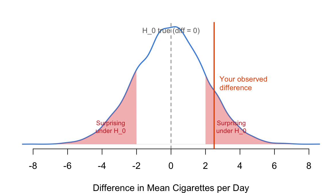
Figure 5.2: A conceptual sampling distribution under $H_0$. The observed difference (red line) is compared to what we’d expect by chance.

In practice, you never draw thousands of samples — that would be impossibly expensive. Instead, statistical theory (the t-distribution, F-distribution, etc.) tells us the shape of the sampling distribution mathematically. R handles all of this for you. Your job is to understand what the p-value means and use it to make a decision.

5.2.2.6 The 4-Step Process

Every hypothesis test follows the same four steps. Commit these to memory — you will use them in Chapters 5 through 11:

State the hypotheses. Write down $H_0$ and $H_a$ in words and in symbols.
Choose a sample and test. Pick an appropriate statistical test based on your variable types (C→Q = t-test/ANOVA, C→C = Chi-Square, etc.).
Assess the evidence. Run the test in R and extract the p-value. Ask: is p < 0.05?
Draw a conclusion. Reject $H_0$ and accept $H_a$, or fail to reject $H_0$. Write your conclusion in plain language.

The remaining chapters in Part II will walk you through a different test for each variable-type combination. The 4-step process is the constant that ties them all together.

5.2.2.7 Frame Your Hypothesis

Before we write the code, let’s make this concrete for your own research project. Take two minutes to write down the hypotheses for your research question.

Exercise 5.1

Your Turn: Frame Your Hypothesis

Think about your own research question — the one you chose at the beginning of this book. If you have not settled on one yet, here are some examples to work with:

Is screen time associated with sleep quality among high school students?
Do left-handed and right-handed people differ in reaction time?
Is a country’s GDP associated with its life expectancy?

Now answer these four questions for your project:

What are your two main variables? Name them. What type is each (categorical or quantitative)?
What is your research question? Write it as a question a friend could understand.
What is your null hypothesis ($H_0$)? Write it in words: “There is no relationship between…”
What is your alternative hypothesis ($H_a$)? Write it in words: “There is a relationship between…”

Keep these hypotheses somewhere you can see them. You will test them in code very shortly.

5.2.3 Code

5.2.3.1 Step 1: State the Hypotheses

$H_0$: Among young adult daily smokers, there is no difference in mean daily cigarette consumption between those with and without major depression ($\mu_{\text{depression}} = \mu_{\text{no depression}}$).

$H_a$: Among young adult daily smokers, there is a difference in mean daily cigarette consumption between those with and without major depression ($\mu_{\text{depression}} \neq \mu_{\text{no depression}}$).

5.2.3.2 Step 2: Choose the Test

We have a categorical explanatory variable (depression: yes/no) and a quantitative response variable (cigarettes per day). That is a C→Q relationship. The appropriate test for comparing the means of two independent groups is an independent samples t-test.

When comparing more than two groups (like mean cigarettes across five ethnicities), you would use ANOVA (Chapter 6). The logic is identical — only the test changes.

5.2.3.3 Step 3: Estimate the Evidence

The R function for a two-sample t-test is t.test(). We specify the relationship using the formula syntax: response ~ explanatory.

# Independent samples t-test — compare means of two independent groups
# ← REPLACE: response_var ~ explanatory_var,   data = your_data_frame
t.test(DailyCigsSmoked ~ MajorDepression,        # formula: numeric ~ categorical
       data = nesarc,                            # the data frame
       var.equal = TRUE)                         # assume equal variance in both groups

## 
##  Two Sample t-test
## 
## data:  DailyCigsSmoked by MajorDepression
## t = -1.3692, df = 1313, p-value = 0.1712
## alternative hypothesis: true difference in means between group No Depression and group Yes Depression is not equal to 0
## 95 percent confidence interval:
##  -1.7938413  0.3191162
## sample estimates:
##  mean in group No Depression mean in group Yes Depression 
##                     13.16632                     13.90368

Let us walk through this output line by line — you will see similar output in every chapter from here on:

data: DailyCigsSmoked by MajorDepression — confirms which variables we are testing. Cigarettes per day, compared across depression groups.

t = -0.92792 — the test statistic. The t-statistic measures how many standard errors our observed difference is from zero. A t-statistic near zero means the difference is small relative to the variability in the data. The sign (negative) simply means the first group alphabetically (“No Depression”) had the lower mean.

df = 1313 — degrees of freedom. Roughly, this is the sample size minus the number of groups. It determines which t-distribution R uses to calculate the p-value. You do not need to calculate this by hand.

p-value = 0.3537 — this is the number you care about. The p-value is 0.35, meaning: if depression and smoking were truly unrelated in the population, there is about a 35% chance that a random sample would produce a difference at least as large as the one we observed. That is not rare at all.

95 percent confidence interval: (-1.180712, 0.420921) — we are 95% confident that the true difference in population means lies between about -1.2 and +0.4 cigarettes per day. Because this interval contains 0 (the null hypothesis value), it agrees with the p-value: the data are consistent with no real difference.

sample estimates — the actual means: 13.17 and 13.55 cigarettes per day. The difference is about 0.38 cigarettes. The footnote “No Depression” appears as the first group because R processes factor levels alphabetically by default.

What does var.equal = TRUE mean? This tells R to assume the two groups have roughly equal variance — the spread of values within each group. When variances are equal, R pools them together to compute a more precise estimate of the standard error. Setting var.equal = FALSE (which is actually R’s default) runs Welch’s t-test, which does not assume equal variance. Which should you use? Check the standard deviations from your earlier tapply() output — the no-depression group has SD ≈ 8.0 and the depression group has SD ≈ 7.7. These are similar, so var.equal = TRUE is reasonable. If one group’s SD were more than double the other’s, you would want var.equal = FALSE. In practice, Welch’s t-test is safer and is the default in R. If you forget and leave it at FALSE (the default), R still gives you a valid result — it simply makes a slightly different assumption about spread. The p-values from both versions are usually very close.

5.2.3.4 Clean Output with `broom::tidy()`

The default t.test() output is a wall of text. For a report, you want a clean table. The broom package’s tidy() function converts any test output into a tidy data frame — one row per result, one column per statistic:

# broom::tidy() + kable() — clean, report-ready results table
# ← REPLACE: response_var ~ explanatory_var
library(broom)                                                        # for tidy()
test <- t.test(DailyCigsSmoked ~ MajorDepression,                     # the t-test
               data = nesarc, var.equal = TRUE)
tidy(test) %>%                                                        # convert to data frame
  select(estimate1, estimate2, statistic, p.value, parameter,         # keep key columns
         conf.low, conf.high) %>%
  knitr::kable(digits = 2,                                            # format as clean table
               caption = "T-test: Daily Cigarettes by Depression")    # ← REPLACE: your title

Table 5.2: T-test: Daily Cigarettes by Depression
estimate1	estimate2	statistic	p.value	parameter	conf.low	conf.high
13.17	13.9	-1.37	0.17	1313	-1.79	0.32

The output is a data frame with columns for the estimate (difference between means), statistic (t-value), p.value, parameter (df), conf.low, and conf.high. This is the format you want for your project report — copy it directly into a table.

broom::tidy() works with almost every statistical test in R: t.test(), cor.test(), chisq.test(), aov(), lm() — you will use it throughout Chapters 6–11.

Do you have to use tidy()? Not at all. The raw output from t.test() contains the same numbers. When you are exploring data and just need to see the p-value, run t.test(...) directly and read the output in the Console — it is faster and perfectly fine for your own understanding. The tidy() + kable() combination is for when you are preparing a final report, poster, or paper — it turns messy output into a table your reader can actually read. For quick checks during analysis, the raw output is all you need.

5.2.3.5 Extracting Just the p-Value

In reports, you often want to pull out just the p-value programmatically rather than copying it from the output:

# Extract just the p-value from the test result
# ← REPLACE: response_var ~ explanatory_var
test_result <- t.test(DailyCigsSmoked ~ MajorDepression,
                      data = nesarc, var.equal = TRUE)  # store the result
test_result$p.value   # ← REPLACE: access the p-value (or $conf.int, $estimate)

## [1] 0.1711689

The $ operator extracts a single component from the test result. Here we take just $p.value. Equally useful: test_result$conf.int for the confidence interval and test_result$estimate for the group means.

5.2.3.6 Step 4: Draw a Conclusion

The p-value is 0.35, which is greater than 0.05. Therefore, we fail to reject the null hypothesis. The observed difference of 0.38 cigarettes per day is easily explained by sampling variation. We do not have sufficient evidence to conclude that depression is associated with cigarette consumption among young adult daily smokers.

Does “failing to reject” mean your project failed? Absolutely not. A null result is still a result worth reporting. Finding that depression and smoking quantity are not detectably related among young adults is useful knowledge — it tells future researchers where to look and where not to. Science advances as much by ruling things out as by discovering new effects. Many of the most important findings in history began with a null result that forced researchers to rethink their assumptions. Report your null result clearly and with confidence — it is honest science, and honesty is what statistics demands.

5.2.3.7 Writing Up Your Results

When you write up a hypothesis test for a report or poster (Chapter 12, Appendix B), include all the essential information in one sentence:

An independent samples t-test found no significant difference in daily cigarette consumption between young adult daily smokers with major depression (M = 13.55, SD = 7.72) and those without depression (M = 13.17, SD = 8.00), t(1313) = -0.93, p = 0.35.

This is the standard format: test name, group means and SDs, test statistic with degrees of freedom, and the p-value. Practice writing results in this format every time — it will become second nature.

5.2.4 Interpretation

5.2.4.1 How to Read the Output — A Quick Reference

For any hypothesis test output in R, find these three numbers:

What to Find	Where It Is	What It Tells You
Test statistic	`t = ...` (or `F = ...`, `$\chi^2$ = ...`)	How large the effect is relative to noise. Larger absolute value = stronger signal.
p-value	`p-value = ...`	The probability of getting data this extreme if $H_0$ were true. The star of the show.
Group estimates	`mean of ...` at the bottom	The actual numbers so you can describe the effect in plain language.

Golden rule: the p-value tells you whether there is an effect. The group estimates (means, proportions, correlation) tell you how big and in what direction.

5.2.4.2 What the p-Value Is NOT

Before you write up your results, clear up the most common misconceptions:

The p-value is NOT the probability that $H_0$ is true. It is the probability of the data, assuming $H_0$ is true. These are different things, and confusing them leads to wrong conclusions.
A large p-value does NOT prove $H_0$ is true. It only means the evidence against $H_0$ is weak. The true difference could be zero, or it could be real but too small for your sample to detect.
A small p-value does NOT mean a large, important effect. With a huge sample size, even a tiny difference can produce a small p-value. In our NESARC data (n = 1,320), a difference of 0.38 cigarettes per day was not significant. But if we had a million respondents, that same 0.38 difference might reach p < 0.001. The p-value measures evidence against the null, not practical importance.
p < 0.05 is not “proof.” It is a convention. A p-value of 0.049 and 0.051 are nearly identical in what they tell you about the evidence. Do not treat 0.05 as a magic cutoff that separates truth from fiction.

5.2.4.3 Common Mistakes Students Make

Confusing statistical significance with practical significance. A significant p-value means the effect probably exists — it does not mean the effect matters. Always report the actual group means so your reader can judge whether the difference is important. How do you judge practical importance? There is no R function for this — it requires thinking about the real world. Ask yourself: would this difference change how anyone thinks or acts? If depressed smokers average 13.5 cigarettes and non-depressed smokers average 13.2, does a 0.3-cigarette gap matter? Probably not. But if a tutoring program raises test scores by 15 points on a 100-point scale, that matters a lot. In Chapter 6, you will also learn about effect sizes like Cohen’s d — standardized numbers that tell you how large a difference is regardless of the measurement units, making it easier to compare across studies.
Running a test before looking at the data. Always graph your data first (Chapter 4). A boxplot or violin plot will tell you immediately whether there is a visible difference between groups. The hypothesis test formalizes what your eyes already suspect.
Forgetting to check variable types before choosing a test. C→Q uses t-test or ANOVA. C→C uses Chi-Square. Q→Q uses correlation or regression. Running the wrong test gives meaningless output that R will not warn you about.
Cherry-picking tests to get p < 0.05. Running five different tests on the same data and reporting only the significant one is called p-hacking. It inflates your false positive rate and undermines the validity of your conclusions. Decide on your test before you see the results.
Ignoring the confidence interval. The p-value says “is there an effect?” The confidence interval says “how big could the effect be, and in which direction?” Always report both. In our example, the 95% CI is (-1.18, 0.42) — the true difference could be anywhere from -1.2 (depressed smokers smoke less) to +0.4 (they smoke more). That wide range tells you the data simply cannot pinpoint the true difference.
Writing “accept the null hypothesis.” You never accept $H_0$. You only “fail to reject” it. The distinction matters: if a jury returns “not guilty,” that does not mean the defendant was proven innocent — only that the evidence was insufficient for a conviction.

5.2.4.4 What Comes Next

You have just learned the framework that powers every chapter in Part II of this book. The specific tests change, but the logic never does: state $H_0$ and $H_a$, choose a test, compute the p-value, draw a conclusion.

In Chapter 6 (ANOVA), you will extend this framework to compare means across three or more groups — for example, does daily cigarette consumption differ across five ethnic groups? The null hypothesis becomes “all group means are equal,” the test statistic changes from t to F, and R provides a new function (aov()). But the 4-step process? Exactly the same.

5.2.5 Hypothesis Tests Reference

You have now seen one test in depth — the two-sample t-test for comparing two means. But hypothesis testing is a family of tools, and you need the right one for your research question. This section is your quick reference. For each test, you will find: what it’s for, the hypotheses in symbols, the R function, and a worked example.

5.2.5.1 Overview Table

Test	Data Type	$H_0$	R Function
1-Sample z-Test for $p$	One sample proportion vs. a claimed value	$p = p_0$	`prop.test(x, n, p = p_0, correct = FALSE)`
2-Sample z-Test for $p_1 - p_2$	Two independent proportions	$p_1 = p_2$	`prop.test(c(x1, x2), c(n1, n2), correct = FALSE)`
1-Sample t-Test for $\mu$	One sample mean vs. a claimed value	$\mu = \mu_0$	`t.test(x, mu = mu_0)`
2-Sample t-Test for $\mu_1 - \mu_2$	Two independent group means	$\mu_1 = \mu_2$	`t.test(y ~ group, data = df, var.equal = TRUE)`
Paired t-Test for $\mu_D$	Paired differences (same subjects, two measurements)	$\mu_D = 0$	`t.test(x, y, paired = TRUE)`

The 4-step process (state hypotheses → choose test → assess evidence → draw conclusion) applies to every one of these. Only the test function and the hypotheses change.

5.2.5.2 1. One-Sample z-Test for a Proportion ($p$)

When to use: You have a single categorical variable (Yes/No, Success/Failure) and you want to test whether the population proportion equals a specific value. For example: “Is the proportion of young adult daily smokers with major depression equal to 0.15 (15%)?”

$H_0$: $p = p_0$ (the population proportion equals the claimed value) $H_a$: $p \neq p_0$ (the population proportion differs)

# 1-sample z-test for a proportion — ← REPLACE: x, n, p = your values
# Test if the proportion with depression differs from 0.15 (15%)

# Count how many have depression in our NESARC subset
n_depression <- sum(nesarc$MajorDepression == "Yes Depression")   # count of "successes"
n_total <- nrow(nesarc)                                           # total sample size

# Run the test
prop_test <- prop.test(x = n_depression,    # number of "successes"
                       n = n_total,         # total sample size
                       p = 0.15,            # ← REPLACE: your hypothesized proportion
                       correct = FALSE)     # no continuity correction (standard z-test)

# Clean results table
library(broom)
tidy(prop_test) %>%                         # convert to data frame
  knitr::kable(digits = 3,                  # format as clean table
               caption = "1-Sample Proportion Test: Depression Rate vs. 15%")

Table 5.3: 1-Sample Proportion Test: Depression Rate vs. 15%
estimate	statistic	p.value	parameter	conf.low	conf.high	method	alternative
0.269	146.459	0	1	0.246	0.294	1-sample proportions test without continuity correction	two.sided

The output gives you the sample proportion, the z-statistic (as $\chi^2$), the p-value, and a confidence interval for the true proportion. correct = FALSE gives the standard z-test; correct = TRUE applies Yates’ continuity correction (more conservative).

5.2.5.3 2. Two-Sample z-Test for Difference of Proportions ($p_1 - p_2$)

When to use: You have a categorical response (Yes/No) and a categorical explanatory variable (two groups). You want to test whether the proportions differ between the two groups. For example: “Is the proportion with depression different for females vs. males among young adult daily smokers?”

$H_0$: $p_1 = p_2$ (the two population proportions are equal) $H_a$: $p_1 \neq p_2$ (the proportions differ)

# 2-sample z-test for difference of proportions — ← REPLACE: your counts and groups
# Test if depression proportion differs by sex

# Build a 2×2 table: Depression (Yes/No) by Sex (Female/Male)
dep_table <- table(nesarc$MajorDepression, nesarc$Sex)            # rows=depression, cols=sex
dep_table                                                         # view the table

##                 
##                  Female Male
##   No Depression     512  453
##   Yes Depression    134  221

# Run the test
prop_test <- prop.test(dep_table,           # the contingency table
                       correct = FALSE)     # standard z-test (no continuity correction)

# Clean results table
library(broom)
tidy(prop_test) %>%                         # convert to data frame
  knitr::kable(digits = 3,                  # format as clean table
               caption = "2-Sample Proportion Test: Depression Rate by Sex")

Table 5.4: 2-Sample Proportion Test: Depression Rate by Sex
estimate1	estimate2	statistic	p.value	parameter	conf.low	conf.high	method	alternative
0.531	0.377	24.345	0	1	0.094	0.213	2-sample test for equality of proportions without continuity correction	two.sided

The output shows the sample proportions for each group, the $\chi^2$ test statistic (which equals $z^2$ for a two-sided test), the p-value, and a confidence interval for the difference in proportions.

5.2.5.4 3. One-Sample t-Test for a Mean ($\mu$)

When to use: You have a single quantitative variable and you want to test whether the population mean equals a specific value. For example: “Do young adult daily smokers smoke 10 cigarettes per day on average?”

$H_0$: $\mu = \mu_0$ (the population mean equals the claimed value) $H_a$: $\mu \neq \mu_0$ (the population mean differs)

# 1-sample t-test for a mean — ← REPLACE: x, mu = your values
# Test if mean daily cigarettes differs from 10

t_test <- t.test(nesarc$DailyCigsSmoked,      # ← REPLACE: your quantitative variable
                 mu = 10,                      # ← REPLACE: your hypothesized mean
                 conf.level = 0.95)            # 95% confidence level (default)

# Clean results table
library(broom)
tidy(t_test) %>%                              # convert to data frame
  knitr::kable(digits = 3,                    # format as clean table
               caption = "1-Sample t-Test: Mean Cigarettes vs. 10 per Day")

Table 5.5: 1-Sample t-Test: Mean Cigarettes vs. 10 per Day
estimate	statistic	p.value	parameter	conf.low	conf.high	method	alternative
13.364	14.092	0	1314	12.896	13.833	One Sample t-test	two.sided

The output gives the sample mean, the t-statistic, degrees of freedom, p-value, and a confidence interval for the true population mean.

5.2.5.5 4. Two-Sample t-Test for Difference of Means ($\mu_1 - \mu_2$)

This is the test we walked through in detail earlier in this chapter — comparing mean cigarette consumption by depression status. Here is the complete code for quick reference:

# 2-sample t-test for difference of means — ← REPLACE: y ~ group
t_test <- t.test(DailyCigsSmoked ~ MajorDepression,   # formula: numeric ~ categorical
                 data = nesarc,                        # the data frame
                 var.equal = TRUE)                     # assume equal variance

# Clean results table
library(broom)
tidy(t_test) %>%                                      # convert to data frame
  select(estimate1, estimate2, statistic, p.value,     # keep key columns
         parameter, conf.low, conf.high) %>%
  knitr::kable(digits = 2,                            # format as clean table
               caption = "2-Sample t-Test: Cigarettes by Depression")

Table 5.6: 2-Sample t-Test: Cigarettes by Depression
estimate1	estimate2	statistic	p.value	parameter	conf.low	conf.high
13.17	13.9	-1.37	0.17	1313	-1.79	0.32

5.2.5.6 5. Paired t-Test for Mean Difference ($\mu_D$)

When to use: You have two quantitative measurements taken on the same subjects — before and after a treatment, left hand vs. right hand, two methods applied to the same person. The pairing matters because each subject serves as their own control, reducing variability. For example: “Does a study technique improve test scores when the same students take a test before and after learning the technique?”

$H_0$: $\mu_D = 0$ (the mean difference in the population is zero — no effect) $H_a$: $\mu_D \neq 0$ (the mean difference is not zero)

# Paired t-test — ← REPLACE: x, y with your two paired measurements
# Using R's built-in sleep dataset: 10 patients, two sleep drugs (paired by patient)

data(sleep)                                     # load the built-in dataset
# sleep$extra = hours of extra sleep vs baseline
# sleep$group = 1 (drug 1) or 2 (drug 2)
# Each patient appears in both groups — measurements are paired

# Extract the two paired measurements
drug1 <- sleep$extra[sleep$group == 1]          # ← REPLACE: your first measurement
drug2 <- sleep$extra[sleep$group == 2]          # ← REPLACE: your second measurement

# Paired t-test — compare the two measurements within each subject
t_test <- t.test(drug1, drug2, paired = TRUE)   # paired = TRUE is the key argument

# Clean results table
library(broom)
tidy(t_test) %>%                                # convert to data frame
  knitr::kable(digits = 3,                      # format as clean table
               caption = "Paired t-Test: Extra Sleep Hours (Drug 1 vs. Drug 2)")

Table 5.7: Paired t-Test: Extra Sleep Hours (Drug 1 vs. Drug 2)
estimate	statistic	p.value	parameter	conf.low	conf.high	method	alternative
-1.58	-4.062	0.003	9	-2.46	-0.7	Paired t-test	two.sided

The output shows the mean of the differences (not the two individual means), the t-statistic, degrees of freedom (n - 1, where n is the number of pairs), and the p-value. If p < 0.05, the difference between the paired measurements is statistically significant.

Key distinction: A paired t-test is NOT the same as a two-sample t-test on the same data. The paired test has more power because it accounts for the fact that the two measurements come from the same person, eliminating between-subject variability.

5.2.5.7 Putting It All Together: Which Test?

Here is a decision flowchart to help you choose the right test for your research question:

Is your response variable categorical (Yes/No)?
- One group? → 1-sample z-test for proportions (prop.test(x, n, p = p0))
- Two groups? → 2-sample z-test for proportions (prop.test(table))
- Three or more groups? → Chi-Square Test of Independence (Chapter 7)
Is your response variable quantitative (numbers)?
- One group, one measurement? → 1-sample t-test (t.test(x, mu = mu0))
- Two independent groups? → 2-sample t-test (t.test(y ~ group))
- Two measurements on the same subjects? → Paired t-test (t.test(x, y, paired = TRUE))
- Three or more groups? → ANOVA (Chapter 6)

Statistics Manual of Haidian Foreign Language School

Chapter 5 Hypothesis Testing

5.1 TL;DR: Hypothesis Testing

5.2 Deep Dive: Hypothesis Testing

5.2.1 Motivating Example

5.2.2 Theory

5.2.2.1 The Logic of Hypothesis Testing

5.2.2.2 The Null Hypothesis (\(H_0\)) and Alternative Hypothesis (\(H_a\))

5.2.2.3 The p-Value

5.2.2.4 The Significance Level (\(\alpha\))

5.2.2.5 Where Does the p-Value Come From? Sampling Distributions

5.2.2.6 The 4-Step Process

5.2.2.7 Frame Your Hypothesis

5.2.3 Code

5.2.3.1 Step 1: State the Hypotheses

5.2.3.2 Step 2: Choose the Test

5.2.3.3 Step 3: Estimate the Evidence

5.2.3.4 Clean Output with `broom::tidy()`

5.2.3.5 Extracting Just the p-Value

5.2.3.6 Step 4: Draw a Conclusion

5.2.3.7 Writing Up Your Results

5.2.4 Interpretation

5.2.4.1 How to Read the Output — A Quick Reference

5.2.4.2 What the p-Value Is NOT

5.2.4.3 Common Mistakes Students Make

5.2.4.4 What Comes Next

5.2.5 Hypothesis Tests Reference

5.2.5.1 Overview Table

5.2.5.2 1. One-Sample z-Test for a Proportion (\(p\))

5.2.5.3 2. Two-Sample z-Test for Difference of Proportions (\(p_1 - p_2\))

5.2.5.4 3. One-Sample t-Test for a Mean (\(\mu\))

5.2.5.5 4. Two-Sample t-Test for Difference of Means (\(\mu_1 - \mu_2\))

5.2.5.6 5. Paired t-Test for Mean Difference (\(\mu_D\))

5.2.5.7 Putting It All Together: Which Test?

Test	Data Type	\(H_0\)	R Function
1-Sample z-Test for \(p\)	One sample proportion vs. a claimed value	\(p = p_0\)	`prop.test(x, n, p = p_0, correct = FALSE)`
2-Sample z-Test for \(p_1 - p_2\)	Two independent proportions	\(p_1 = p_2\)	`prop.test(c(x1, x2), c(n1, n2), correct = FALSE)`
1-Sample t-Test for \(\mu\)	One sample mean vs. a claimed value	\(\mu = \mu_0\)	`t.test(x, mu = mu_0)`
2-Sample t-Test for \(\mu_1 - \mu_2\)	Two independent group means	\(\mu_1 = \mu_2\)	`t.test(y ~ group, data = df, var.equal = TRUE)`
Paired t-Test for \(\mu_D\)	Paired differences (same subjects, two measurements)	\(\mu_D = 0\)	`t.test(x, y, paired = TRUE)`

Chapter 5 Hypothesis Testing

5.1 TL;DR: Hypothesis Testing

5.2 Deep Dive: Hypothesis Testing

5.2.1 Motivating Example

5.2.2 Theory

5.2.2.1 The Logic of Hypothesis Testing

5.2.2.2 The Null Hypothesis (\(H_0\)) and Alternative Hypothesis (\(H_a\))

5.2.2.3 The p-Value

5.2.2.4 The Significance Level (\(\alpha\))

5.2.2.5 Where Does the p-Value Come From? Sampling Distributions

5.2.2.6 The 4-Step Process

5.2.2.7 Frame Your Hypothesis

5.2.3 Code

5.2.3.1 Step 1: State the Hypotheses

5.2.3.2 Step 2: Choose the Test

5.2.3.3 Step 3: Estimate the Evidence

5.2.3.4 Clean Output with broom::tidy()

5.2.3.5 Extracting Just the p-Value

5.2.3.6 Step 4: Draw a Conclusion

5.2.3.7 Writing Up Your Results

5.2.4 Interpretation

5.2.4.1 How to Read the Output — A Quick Reference

5.2.4.2 What the p-Value Is NOT

5.2.4.3 Common Mistakes Students Make

5.2.4.4 What Comes Next

5.2.5 Hypothesis Tests Reference

5.2.5.1 Overview Table

5.2.5.2 1. One-Sample z-Test for a Proportion (\(p\))

5.2.5.3 2. Two-Sample z-Test for Difference of Proportions (\(p_1 - p_2\))

5.2.5.4 3. One-Sample t-Test for a Mean (\(\mu\))

5.2.5.5 4. Two-Sample t-Test for Difference of Means (\(\mu_1 - \mu_2\))

5.2.5.6 5. Paired t-Test for Mean Difference (\(\mu_D\))

5.2.5.7 Putting It All Together: Which Test?

5.2.3.4 Clean Output with `broom::tidy()`