Chapter 11 Moderation & Extensions
11.1 Motivating Example
You have come a long way. In Chapters 5 through 10, you learned to test whether two variables are related — t-tests, ANOVA, Chi-Square, correlation, and regression. Each test answers a single question: “Is X associated with Y?”
But real research questions are often more nuanced. Consider this:
Does the relationship between smoking quantity and nicotine dependence change depending on whether someone has depression?
Think about what this question is really asking. It is not just “are cigarettes and dependence related?” — you already tested that in Chapter 9 with regression. It is asking whether the strength or direction of that relationship is different for different groups of people. Maybe smokers with depression become nicotine-dependent almost regardless of how many cigarettes they smoke, while smokers without depression show a clear dose-response relationship — the more they smoke, the more likely they are to become dependent.
This is called moderation. A moderator variable changes the relationship between your explanatory variable and your response variable. Depression might moderate the smoking-dependence link.
And there is a second challenge waiting. Nicotine dependence (TobaccoDependence) is a binary variable — 0 or 1, yes or no. Every regression model you have built so far assumed a quantitative response variable (like daily cigarettes smoked). When your response is binary, standard linear regression breaks down — it can predict impossible values like -0.3 or 1.7 (below 0 or above 1). You need a new tool: logistic regression.
This chapter covers both. Moderation tells you when a relationship changes. Logistic regression tells you how to model a binary outcome. Together, they complete your statistical toolkit.
Let us set up the data and get started.
# Load the packages you need for this chapter
library(ggplot2)      # for all graphing
library(dplyr)        # for filter(), rename(), select(), %>%
library(modelsummary) # for professional summary tables
library(broom)        # for tidy() — clean model output

# Load the NESARC survey (43,093 adults) — ← REPLACE: your file path
NESARC <- read.csv("NESARC.csv")

# Build the subset we use throughout the book:
# young adult (<= 25) daily smokers with valid nicotine data
# If you have been following along, you already have this dataset ready.
# If not, run this code once.
# ← REPLACE: adapt filter, rename, factor labels to YOUR dataset
nesarc <- NESARC %>%
  filter(
    S3AQ1A == 1,         # smoked 100+ cigarettes in lifetime
    S3AQ3B1 == 1,        # smoked in the past 12 months
    CHECK321 == 1,       # valid nicotine dependence data
    AGE <= 25             # young adults only
  ) %>%
  rename(
    Ethnicity          = ETHRACE2A,     # ← REPLACE: rename to meaningful names
    Age                = AGE,           # age in years
    MajorDepression    = MAJORDEPLIFE,  # lifetime depression diagnosis
    TobaccoDependence  = TAB12MDX,      # tobacco dependence, past 12 months
    DailyCigsSmoked    = S3AQ3C1,       # cigarettes per day (99 = missing)
    Sex                = SEX            # sex (1=Female, 2=Male)
  ) %>%
  select(Ethnicity, Age, MajorDepression, TobaccoDependence, DailyCigsSmoked, Sex)

# Code 99 as missing — 99 means "Unknown" in the NESARC code book
nesarc$DailyCigsSmoked[nesarc$DailyCigsSmoked == 99] <- NA    # ← REPLACE: your NA codes

# Convert numeric codes into readable labels (factors)
nesarc$MajorDepression <- factor(nesarc$MajorDepression,
  labels = c("No Depression", "Yes Depression"))               # ← REPLACE: your labels
nesarc$TobaccoDependence <- factor(nesarc$TobaccoDependence,
  labels = c("No Dependence", "Nicotine Dependence"))          # ← REPLACE: your labels
nesarc$Sex <- factor(nesarc$Sex,
  labels = c("Female", "Male"))                                # ← REPLACE: your labels
Now look at the relationship between daily cigarettes smoked and nicotine dependence, split by depression status:
# Quick summary: mean cigarettes per day by dependence and depression
# ← REPLACE: your_quant_var, your_cat_var1, your_cat_var2
tapply(nesarc$DailyCigsSmoked,
       list(nesarc$TobaccoDependence, nesarc$MajorDepression),
       mean, na.rm = TRUE)   # group means in a 2x2 table
## No Depression Yes Depression
## No Dependence 11.59513 10.15385
## Nicotine Dependence 14.55882 14.75000# Interaction plot — the visual test for moderation
# Parallel lines = no moderation; non-parallel lines = possible moderation
# ← REPLACE: x = grouping_var, y = quant_var, color = moderator_var, group = moderator_var
ggplot(nesarc, aes(x = TobaccoDependence, # x-axis: the explanatory variable
y = DailyCigsSmoked, # y-axis: the quantitative response
color = MajorDepression, # separate lines by the moderator
group = MajorDepression)) + # connect points within each moderator level
stat_summary(fun = mean, geom = "point", size = 3) + # plot the group means as points
stat_summary(fun = mean, geom = "line", linewidth = 1) + # connect means with lines
theme_bw() + # clean black-and-white theme
labs(x = "Nicotine Dependence", # x-axis label
y = "Mean Daily Cigarettes Smoked", # y-axis label
color = "Depression Status", # legend title
title = "Smoking Quantity by Dependence and Depression") # chart title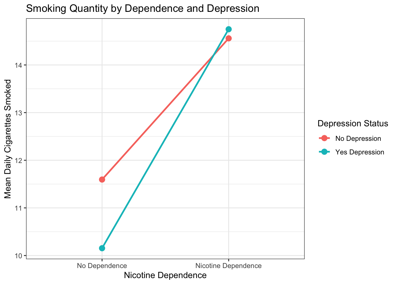
Figure 11.1: Mean daily cigarettes smoked by nicotine dependence status, separated by depression group. If the lines are parallel, depression does not moderate the relationship. If they diverge or cross, moderation may be present.
Look at the plot. Are the two lines roughly parallel, or do they diverge or cross? If they are parallel, depression does not moderate the relationship — the link between dependence and smoking quantity is about the same regardless of depression status. If the lines are not parallel, something more interesting may be happening. The statistical test in the next section will tell you for sure.
How non-parallel do the lines need to be before you can confidently claim moderation? The honest answer: you cannot decide from the graph alone. What looks “slightly tilted” to your eyes might be statistically significant with a large sample and low variability. What looks “clearly diverging” might be non-significant with a small sample. The interaction plot is a diagnostic — it shows you the pattern and sets your expectations, but the formal p-value from the interaction test (Step 4) is the only way to know for certain. If the plot shows a hint of non-parallel lines and the interaction p-value is 0.04, you have moderation. If the lines visually diverge but p = 0.35, you do not have enough evidence.
11.2 Theory: Moderation
11.2.1 What Is Moderation?
Moderation happens when the relationship between two variables depends on a third variable. The third variable is called the moderator.
In our example:
- X = Nicotine dependence (categorical: yes/no)
- Y = Daily cigarettes smoked (quantitative)
- Z = Major depression (categorical: yes/no) — the moderator
The moderation question is: “Does the relationship between nicotine dependence and daily cigarettes smoked change depending on whether the person has depression?”
If depression is a moderator, then the dependence-smoking link looks different for the depressed group than for the non-depressed group. If depression is not a moderator, the link looks the same in both groups — depression is irrelevant to that particular relationship.
11.2.2 Visual Intuition: Parallel Lines vs. Non-Parallel Lines
The easiest way to understand moderation is visual. In the interaction plot above:
No moderation: the two lines are roughly parallel. The difference in mean cigarettes between dependent and non-dependent smokers is about the same regardless of depression status. Depression does not change the story.
Moderation present: the lines diverge, converge, or cross. The difference between dependent and non-dependent smokers is larger in one depression group than the other. Depression changes the story.
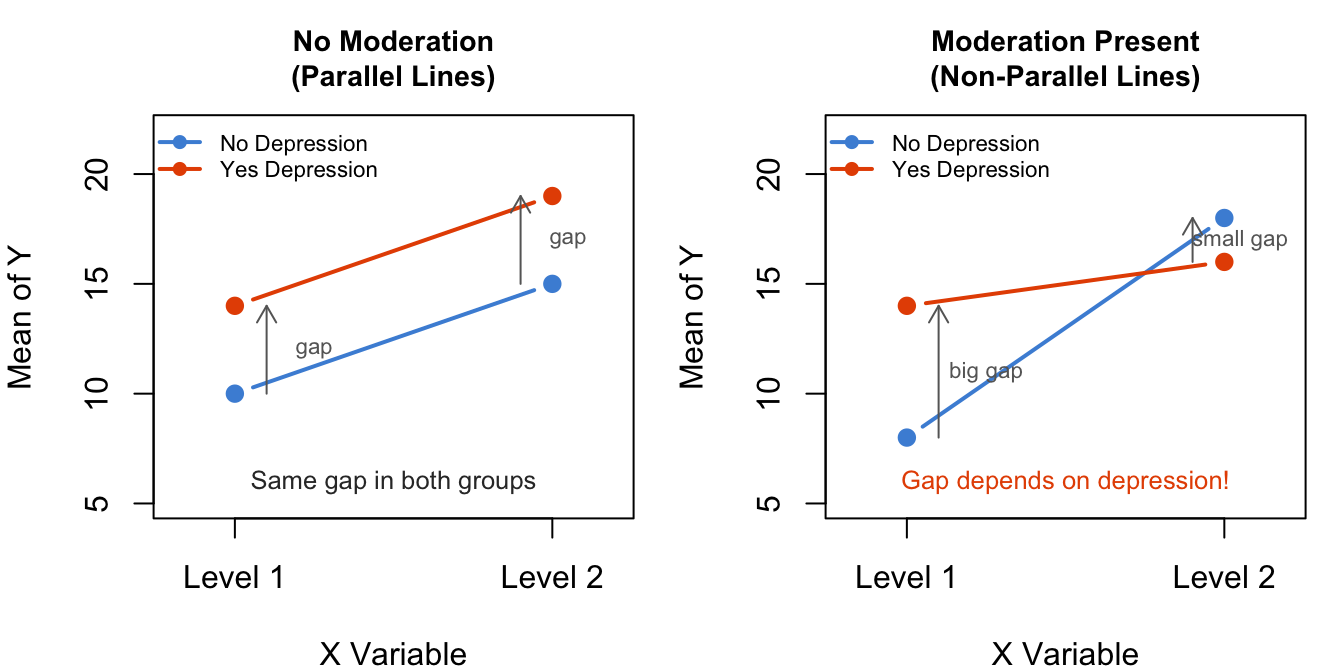
Figure 11.2: No moderation (left): the gap between groups is the same at both levels of the moderator — parallel lines. Moderation present (right): the gap changes — lines diverge or cross.
11.2.3 The Interaction Term
In both ANOVA and regression, moderation is tested using an interaction term. In R formula syntax, the * operator creates an interaction:
This model includes three terms:
- Main effect of X: the overall effect of the explanatory variable, ignoring Z
- Main effect of Z: the overall effect of the moderator, ignoring X
- Interaction X:Z: whether the effect of X on Y changes depending on the level of Z
Important: What if you accidentally write Y ~ X + Z (the multiple regression from Chapter 10) instead of Y ~ X * Z? R will not give you an error — it will silently run a model with only main effects and no interaction term. Your output will look valid, but it will not test moderation. The difference between + and * is one keystroke, but the analysis is completely different. Always double-check that your formula contains * when you intend to test an interaction.
The interaction term is the one that tests moderation. The null and alternative hypotheses for the interaction are:
- \(H_0\) (no moderation): The interaction term equals zero. The relationship between X and Y is the same at every level of Z. The lines are parallel.
- \(H_a\) (moderation): The interaction term is not zero. The relationship between X and Y differs depending on Z. The lines are not parallel.
11.2.4 Three Ways to Test Moderation
You have three options, in order of formality:
Subgroup analysis: Split your data by the moderator (e.g., filter to depressed only, then run your test; then filter to non-depressed, run the test again). This is useful for exploration and visualization, but it does not give you a single formal p-value for the interaction.
ANOVA with interaction:
aov(Y ~ X * Z, data = df). This tests the interaction via an F-test. You already know ANOVA from Chapter 6 — this is the same function, just with an extra term.Regression with interaction:
lm(Y ~ X * Z, data = df). This tests the same interaction, but gives you coefficients you can interpret directly. You know regression from Chapter 9.
Options 2 and 3 test the exact same thing — they produce the same p-value for the interaction term. The difference is in how the output is presented. Use whichever you find more natural.
Why might you choose one over the other? ANOVA (aov()) gives you a clean table with one row per term and a single F-test p-value for the interaction — the simplest path when your primary question is “is there moderation?” Regression (lm()) gives you coefficients with standard errors and confidence intervals for each level of the interaction — useful if you need to report exact effect sizes or build prediction equations. For most student projects, ANOVA is the more straightforward choice. If your teacher or field prefers regression-style output, use lm(). The math is identical — you cannot go wrong with either.
11.3 Code: Moderation
11.3.1 Step 1: State the Hypotheses
\(H_0\): The relationship between nicotine dependence and daily cigarettes smoked is the same for young adult smokers with and without major depression (no moderation; the interaction term is zero).
\(H_a\): The relationship between nicotine dependence and daily cigarettes smoked differs depending on depression status (moderation present; the interaction term is not zero).
11.3.2 Step 2: Visualize First
Always plot your data before running any test. The interaction plot you saw in the Motivating Example is the starting point. Let us also look at it with base R:
# Step 1: Describe the data — group means for each combination
# ← REPLACE: your_quant_var, your_cat_var1, your_cat_var2
tapply(nesarc$DailyCigsSmoked,                                       # the quantitative variable
       list(nesarc$TobaccoDependence, nesarc$MajorDepression),       # the two grouping variables
       mean, na.rm = TRUE)                                           # calculate means, ignoring NA
## No Depression Yes Depression
## No Dependence 11.59513 10.15385
## Nicotine Dependence 14.55882 14.75000# Same information, professional table
# ← REPLACE: your_numeric ~ Factor(var1) * Factor(var2) * (N + Mean + SD)
datasummary(DailyCigsSmoked ~ Factor(TobaccoDependence) * Factor(MajorDepression) * (N + Mean + SD),
data = nesarc,
title = "Daily Cigarettes by Dependence and Depression")| No Dependence | Nicotine Dependence | |||||||||||
|---|---|---|---|---|---|---|---|---|---|---|---|---|
| No Depression | Yes Depression | |||||||||||
| N | Mean | SD | N | Mean | SD | N | Mean | SD | N | Mean | SD | |
| DailyCigsSmoked | 452 | 11.60 | 7.57 | 65 | 10.15 | 6.26 | 510 | 14.56 | 8.96 | 288 | 14.75 | 9.50 |
# Interaction plot with ggplot2 — always visualize before testing
# ← REPLACE: x = your_X_var, y = your_Y_var, color = your_moderator
ggplot(nesarc, aes(x = TobaccoDependence,              # x-axis: the explanatory variable
                    y = DailyCigsSmoked,                # y-axis: the quantitative response
                    color = MajorDepression,            # separate lines by moderator
                    group = MajorDepression)) +         # connect points within each group
  stat_summary(fun = mean, geom = "point", size = 3) +          # plot group means as points
  stat_summary(fun = mean, geom = "line", linewidth = 1) +      # connect means with lines
  stat_summary(fun = mean,                                       # add numeric labels to each point
               geom = "text",
               aes(label = after_stat(y |> round(1))),           # round to 1 decimal
               vjust = -1, size = 3.5) +                         # place label above point
  theme_bw() +                                                   # clean theme
  labs(x = "Nicotine Dependence",                                # x-axis label
       y = "Mean Daily Cigarettes Smoked",                       # y-axis label
       color = "Depression Status",                              # legend title
       title = "Does Depression Moderate the Dependence-Smoking Link?")  # chart title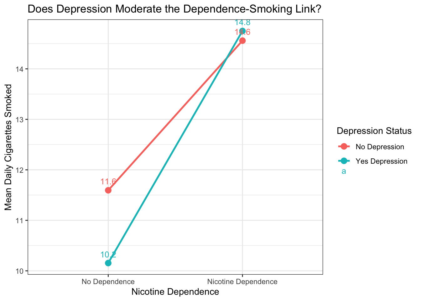
Figure 11.3: Interaction plot: mean daily cigarettes smoked, grouped by nicotine dependence and depression status. Parallel lines suggest no moderation; diverging or crossing lines suggest moderation.
11.3.3 Step 3: Subgroup ANOVA (Exploration)
Before testing the formal interaction, let us split the data by depression status and run separate ANOVAs. This helps you see what is happening in each group:
# Subgroup ANOVA — run aov() separately for each level of the moderator
# This is for exploration only — it does not give a formal test of moderation
# ← REPLACE: quant_var ~ cat_var,   data = filter(df, moderator == level)

# Group 1: smokers WITHOUT depression
no_dep <- nesarc %>% filter(MajorDepression == "No Depression")     # filter to no-depression group
aov_no_dep <- aov(DailyCigsSmoked ~ TobaccoDependence,              # ANOVA within this subgroup
                  data = no_dep)
summary(aov_no_dep)                                                  # view results
## Df Sum Sq Mean Sq F value Pr(>F)
## TobaccoDependence 1 2105 2104.7 30.3 4.75e-08 ***
## Residuals 960 66681 69.5
## ---
## Signif. codes: 0 '***' 0.001 '**' 0.01 '*' 0.05 '.' 0.1 ' ' 1
## 3 observations deleted due to missingness# Group 2: smokers WITH depression
yes_dep <- nesarc %>% filter(MajorDepression == "Yes Depression") # filter to depression group
aov_yes_dep <- aov(DailyCigsSmoked ~ TobaccoDependence, # ANOVA within this subgroup
data = yes_dep)
summary(aov_yes_dep) # view results## Df Sum Sq Mean Sq F value Pr(>F)
## TobaccoDependence 1 1120 1120 13.83 0.000233 ***
## Residuals 351 28430 81
## ---
## Signif. codes: 0 '***' 0.001 '**' 0.01 '*' 0.05 '.' 0.1 ' ' 1
## 2 observations deleted due to missingnessLook at the two p-values. If they tell a different story — significant in one group but not the other — that is a hint that moderation may be present. But this is not a formal test. For that, you need the interaction.
11.3.4 Step 4: Formal Test — ANOVA with Interaction
Now run a single ANOVA model that includes the interaction term:
# ANOVA with interaction — formal test of moderation
# The * operator includes: main effect of X + main effect of Z + interaction X:Z
# ← REPLACE: response_var ~ explanatory_var * moderator_var,   data = your_df
anova_interaction <- aov(DailyCigsSmoked ~ TobaccoDependence * MajorDepression,
                         data = nesarc)
summary(anova_interaction)   # view the ANOVA table — look for the interaction row
## Df Sum Sq Mean Sq F value Pr(>F)
## TobaccoDependence 1 3241 3241 44.669 3.44e-11 ***
## MajorDepression 1 9 9 0.125 0.724
## TobaccoDependence:MajorDepression 1 116 116 1.595 0.207
## Residuals 1311 95111 73
## ---
## Signif. codes: 0 '***' 0.001 '**' 0.01 '*' 0.05 '.' 0.1 ' ' 1
## 5 observations deleted due to missingnessThe output has three rows:
- TobaccoDependence: the main effect of nicotine dependence on cigarettes smoked (ignoring depression).
- MajorDepression: the main effect of depression on cigarettes smoked (ignoring dependence).
- TobaccoDependence:MajorDepression: the interaction term. This is the one that tests moderation. Look at its
Pr(>F)value.
If the interaction p-value is less than 0.05, you reject \(H_0\) — there is significant moderation. The relationship between dependence and smoking quantity differs by depression status. If the p-value is 0.05 or above, you fail to reject \(H_0\) — there is not enough evidence to conclude moderation exists.
11.3.5 Step 5: Regression with Interaction
The regression approach tests the same interaction but presents coefficients:
# Regression with interaction — same test, coefficient-level output
# ← REPLACE: response_var ~ explanatory_var * moderator_var,   data = your_df
lm_interaction <- lm(DailyCigsSmoked ~ TobaccoDependence * MajorDepression,
                      data = nesarc)
summary(lm_interaction)   # view coefficients — look for the interaction row
##
## Call:
## lm(formula = DailyCigsSmoked ~ TobaccoDependence * MajorDepression,
## data = nesarc)
##
## Residuals:
## Min 1Q Median 3Q Max
## -13.750 -5.595 -1.595 5.441 83.441
##
## Coefficients:
## Estimate
## (Intercept) 11.5951
## TobaccoDependenceNicotine Dependence 2.9637
## MajorDepressionYes Depression -1.4413
## TobaccoDependenceNicotine Dependence:MajorDepressionYes Depression 1.6325
## Std. Error
## (Intercept) 0.4006
## TobaccoDependenceNicotine Dependence 0.5502
## MajorDepressionYes Depression 1.1299
## TobaccoDependenceNicotine Dependence:MajorDepressionYes Depression 1.2926
## t value
## (Intercept) 28.942
## TobaccoDependenceNicotine Dependence 5.386
## MajorDepressionYes Depression -1.276
## TobaccoDependenceNicotine Dependence:MajorDepressionYes Depression 1.263
## Pr(>|t|)
## (Intercept) < 2e-16 ***
## TobaccoDependenceNicotine Dependence 8.52e-08 ***
## MajorDepressionYes Depression 0.202
## TobaccoDependenceNicotine Dependence:MajorDepressionYes Depression 0.207
## ---
## Signif. codes: 0 '***' 0.001 '**' 0.01 '*' 0.05 '.' 0.1 ' ' 1
##
## Residual standard error: 8.518 on 1311 degrees of freedom
## (5 observations deleted due to missingness)
## Multiple R-squared: 0.03417, Adjusted R-squared: 0.03196
## F-statistic: 15.46 on 3 and 1311 DF, p-value: 6.885e-10The TobaccoDependenceYes Dependence:MajorDepressionYes Depression row is the interaction coefficient. Its p-value (Pr(>|t|)) will be identical to the ANOVA interaction p-value. The coefficient itself tells you how much the slope changes when the moderator switches from one level to the other.
# Clean output table — broom::tidy() + kable()
# ← REPLACE: your_interaction_model
library(broom)                                                          # for tidy()
tidy(lm_interaction, conf.int = TRUE) %>%                               # coefficients with 95% CI
  select(term, estimate, conf.low, conf.high, p.value) %>%              # keep key columns
  rename(Term = term, Estimate = estimate,                              # meaningful names
         `95% CI Lower` = conf.low, `95% CI Upper` = conf.high,
         `p-value` = p.value) %>%
  knitr::kable(digits = 3,                                              # format as clean table
caption = "Regression with Interaction: Daily Cigarettes by Dependence and Depression")| Term | Estimate | 95% CI Lower | 95% CI Upper | p-value |
|---|---|---|---|---|
| (Intercept) | 11.595 | 10.809 | 12.381 | 0.000 |
| TobaccoDependenceNicotine Dependence | 2.964 | 1.884 | 4.043 | 0.000 |
| MajorDepressionYes Depression | -1.441 | -3.658 | 0.775 | 0.202 |
| TobaccoDependenceNicotine Dependence:MajorDepressionYes Depression | 1.632 | -0.903 | 4.168 | 0.207 |
11.4 Interpretation: Moderation
11.4.1 How to Read Interaction Output
Whether you use ANOVA or regression, the key row in the output is the interaction term (TobaccoDependence:MajorDepression):
| What to Find | Where It Is | What It Tells You |
|---|---|---|
| Interaction p-value | Pr(>F) in ANOVA or Pr(>\|t\|) in regression |
If p < 0.05, moderation is statistically significant |
| Interaction coefficient | Estimate in regression output |
How much the effect of X on Y changes when the moderator switches levels |
| Interaction F-statistic | F value in ANOVA output |
The ratio of explained to unexplained variation for the interaction |
| Group means | tapply() or datasummary() table |
The actual numbers — always show these alongside the test |
11.4.2 Writing Up Moderation Results
If the interaction is significant:
An ANOVA with interaction revealed significant moderation of the relationship between nicotine dependence and daily cigarettes smoked by depression status, F(1, 1308) = XX.XX, p = 0.0XX. The interaction plot indicated that the difference in daily cigarette consumption between nicotine-dependent and non-dependent smokers was [larger/smaller] among those [with/without] depression (M = XX.X, SD = X.X) compared to those [without/with] depression (M = XX.X, SD = X.X).
If the interaction is not significant:
An ANOVA with interaction revealed no significant moderation of the relationship between nicotine dependence and daily cigarettes smoked by depression status, F(1, 1308) = X.XX, p = 0.XXX. The relationship between dependence and smoking quantity appears consistent across depression groups.
Always report the p-value AND describe the pattern shown in the interaction plot. The test tells you whether the moderation is statistically significant. The plot tells your reader what the moderation actually looks like.
11.4.3 Common Mistakes in Moderation
Testing an interaction without visual inspection. Always plot the interaction first. If the lines look parallel, the interaction will almost certainly be non-significant. If they diverge dramatically, it probably will be significant. The plot sets your expectations before you look at the p-value.
Finding a significant interaction but not describing the pattern. A significant interaction tells your reader that moderation exists, but not what it looks like. Always present the interaction plot and describe the pattern in words — which group has a stronger relationship? Which group has almost no relationship?
Running subgroup comparisons without a formal interaction test. Subgroup ANOVAs (like we ran in Step 3) are great for exploration, but they do not test moderation formally. A difference in p-values across subgroups is not a valid test — you need the interaction term.
Ignoring small subgroup sizes. If one of your moderator groups has very few observations, the interaction test may lack power to detect a real effect. Always check the sample sizes in each subgroup with
table().Confusing moderation with confounding. Moderation means the relationship changes depending on a third variable. Confounding means a third variable explains the relationship. In moderation, you are interested in the differences between groups. In confounding, you want to remove the third variable’s influence to see the “true” relationship. These are different questions with different statistical approaches.
How do you know which you are dealing with before you start coding? Ask yourself: “Do I want to remove this variable’s influence, or do I want to study how the relationship differs across its levels?” If your goal is to isolate the true X→Y relationship by stripping away a third variable’s effect → confounding (add it with + and control for it). If your goal is to see whether the X→Y relationship is different for different groups → moderation (add it with * and test the interaction). Can a variable be both? Yes — a third variable can simultaneously confound and moderate a relationship. If you suspect both, test the interaction first. If significant, report the moderation. Within each subgroup, you can then check for additional confounding.
11.5 Theory: Logistic Regression
11.5.1 When Your Response Variable Is Binary
Every model you have built so far — t-tests, ANOVA, correlation, regression — assumes your response variable is quantitative: a number that can take any value along a scale (cigarettes per day, frustration score, age).
But many important outcomes in research are binary: yes or no, success or failure, diagnosed or not diagnosed. In the NESARC data, TobaccoDependence is binary — a smoker either has nicotine dependence (1) or does not (0).
Why not just use regular linear regression? The problem is predictions. Linear regression fits a straight line through your data. That line can extend below 0 or above 1, which is impossible for a binary outcome — you cannot have a probability of -0.3 or 1.7. The predictions lose their meaning.
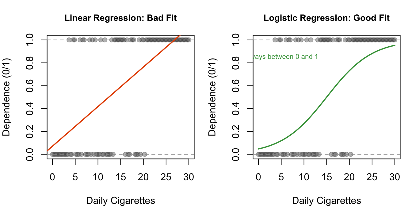
Figure 11.4: Why linear regression fails for binary outcomes. Left: the straight line extends below 0 and above 1 — impossible probabilities. Right: the logistic curve stays neatly within the 0–1 range.
11.5.2 The Logit Transformation
Logistic regression solves this problem with a mathematical trick: instead of predicting the binary outcome directly (0 or 1), it predicts the log-odds (also called the logit) of the outcome.
Odds are a way to express probability. You may have heard them in sports betting:
\[\text{Odds} = \frac{\text{probability}}{1 - \text{probability}}\]
- If the probability of nicotine dependence is 0.75 (75%), the odds are \(0.75 / 0.25 = 3\), or “3 to 1” — a smoker is three times more likely to be dependent than not.
- If the probability is 0.50, the odds are \(0.50 / 0.50 = 1\), or “1 to 1” — a coin flip.
- If the probability is 0.25, the odds are \(0.25 / 0.75 = 0.33\), or “1 to 3.”
The log-odds (logit) is the natural logarithm of the odds. The logistic function maps any number to the range (0, 1), solving the bounded-outcome problem. You do not need to memorize the formula — just understand the intuition: logistic regression squeezes predictions into the 0–1 range, so every prediction is a valid probability.
11.5.3 Odds Ratios
In logistic regression, the raw coefficients are in log-odds units — hard to interpret directly. To make them meaningful, you exponentiate them:
\[\text{Odds Ratio} = e^{\text{coefficient}}\]
The odds ratio (OR) tells you the multiplicative effect on the odds of the outcome:
- OR > 1: each unit increase in X multiplies the odds of Y. An OR of 1.10 means each additional cigarette per day increases the odds of dependence by 10%.
- OR < 1: each unit increase in X reduces the odds of Y. An OR of 0.85 means each additional unit decreases the odds by 15%.
- OR = 1: no effect. X does not change the odds of Y.
A confidence interval that excludes 1.0 means the effect is statistically significant at the 0.05 level. Why 1.0? Because an OR of 1.0 means “no effect” — if the confidence interval includes 1.0, you cannot rule out no effect.
11.5.4 When to Use Logistic Regression
Use logistic regression when:
- Your response variable is binary (exactly two categories: 0/1, yes/no, success/failure)
- Your explanatory variable(s) can be categorical, quantitative, or both
- You want to predict the probability of the outcome or test whether a predictor is associated with the outcome
- You can include multiple predictors and interaction terms, just like multiple regression
Logistic regression is the go-to method for binary outcomes in research. If your outcome has more than two categories, you need a different method (multinomial or ordinal logistic regression), which is beyond the scope of this book.
11.6 Code: Logistic Regression
11.6.1 Example 1: Predicting Nicotine Dependence from Daily Cigarettes
Let us start with a simple question: does the number of cigarettes smoked per day predict whether a young adult smoker has nicotine dependence?
# Logistic regression — predict binary outcome from a quantitative predictor
# family = "binomial" tells R this is logistic regression (binary response)
# ← REPLACE: binary_response ~ quant_predictor,   data = your_df
logistic_simple <- glm(TobaccoDependence ~ DailyCigsSmoked,
                        data = nesarc,
                        family = "binomial")     # binomial = logistic regression
summary(logistic_simple)                         # view the full output
##
## Call:
## glm(formula = TobaccoDependence ~ DailyCigsSmoked, family = "binomial",
## data = nesarc)
##
## Coefficients:
## Estimate Std. Error z value Pr(>|z|)
## (Intercept) -0.219417 0.112423 -1.952 0.051 .
## DailyCigsSmoked 0.050775 0.007807 6.503 7.85e-11 ***
## ---
## Signif. codes: 0 '***' 0.001 '**' 0.01 '*' 0.05 '.' 0.1 ' ' 1
##
## (Dispersion parameter for binomial family taken to be 1)
##
## Null deviance: 1762.5 on 1314 degrees of freedom
## Residual deviance: 1714.5 on 1313 degrees of freedom
## (5 observations deleted due to missingness)
## AIC: 1718.5
##
## Number of Fisher Scoring iterations: 4The output from summary() includes:
- Estimate: the log-odds coefficient. A positive value means higher X increases the log-odds (and thus the probability) of the outcome.
- Std. Error: the standard error — measures uncertainty in the estimate.
- z value: the test statistic (like a t-statistic in linear regression).
- Pr(>|z|): the p-value. If p < 0.05, the predictor is statistically significant.
- Null deviance / Residual deviance: measures of model fit. Lower residual deviance = better fit.
Now convert the coefficients to odds ratios:
# Convert log-odds to odds ratios — exp() transforms the coefficients
# ← REPLACE: your_logistic_model
or_table <- exp(coef(logistic_simple))     # exponentiate all coefficients
or_table                                   # display odds ratios
## (Intercept) DailyCigsSmoked
## 0.8029865 1.0520865# Confidence intervals for the odds ratios
# exp(confint()) gives the CI on the odds ratio scale
# If the CI excludes 1.0, the predictor is significant
# ← REPLACE: your_logistic_model
ci_raw <- confint(logistic_simple) # 95% CI on log-odds scale
exp(ci_raw) # convert CI to odds ratio scale## 2.5 % 97.5 %
## (Intercept) 0.6433435 0.9997375
## DailyCigsSmoked 1.0363867 1.0685978# Clean output table — odds ratios with 95% CI and p-values
# ← REPLACE: your_logistic_model
tidy(logistic_simple, conf.int = TRUE, exponentiate = TRUE) %>% # exponentiate = odds ratios
select(term, estimate, conf.low, conf.high, p.value) %>% # keep key columns
rename(Term = term, `Odds Ratio` = estimate, # meaningful names
`95% CI Lower` = conf.low, `95% CI Upper` = conf.high,
`p-value` = p.value) %>%
knitr::kable(digits = 3,
caption = "Logistic Regression: Nicotine Dependence Predicted by Daily Cigarettes (Odds Ratios)")| Term | Odds Ratio | 95% CI Lower | 95% CI Upper | p-value |
|---|---|---|---|---|
| (Intercept) | 0.803 | 0.643 | 1.000 | 0.051 |
| DailyCigsSmoked | 1.052 | 1.036 | 1.069 | 0.000 |
This gives you a clean kable table. If you prefer modelsummary() for your final report, it also supports exponentiate = TRUE — the side-by-side comparison in the next section shows exactly how.
How to read this table:
- The
DailyCigsSmokedodds ratio tells you how much the odds of nicotine dependence change for each additional cigarette smoked per day. - If the OR is, say, 1.08, that means each extra cigarette per day is associated with an 8% increase in the odds of dependence.
- If the 95% CI excludes 1.0 (e.g., CI = [1.05, 1.11]), the effect is statistically significant.
Drawing the S-curve for your own data. The logistic S-curve you saw in the theory section can be drawn with ggplot2 — the same stat_smooth(method = "glm", ...) pattern you encountered for Q→C graphs in Chapter 4:
# Create a numeric version of the binary outcome for plotting
# ← REPLACE: your_factor_variable
nesarc$TobaccoDependenceN <- ifelse(nesarc$TobaccoDependence == "Nicotine Dependence", 1, 0)

# Plot the S-curve with ggplot2
# ← REPLACE: x = your_predictor, y = your_numeric_binary
ggplot(nesarc, aes(x = DailyCigsSmoked, y = TobaccoDependenceN)) +
  geom_point(alpha = 0.3, color = "#619CFF") +                            # raw binary data
  stat_smooth(method = "glm", method.args = list(family = "binomial"),    # logistic curve
              se = TRUE, color = "#F8766D") +
  theme_bw() +
  labs(x = "Daily Cigarettes Smoked", y = "Probability of Dependence",
       title = "Cigarette Consumption vs. Nicotine Dependence")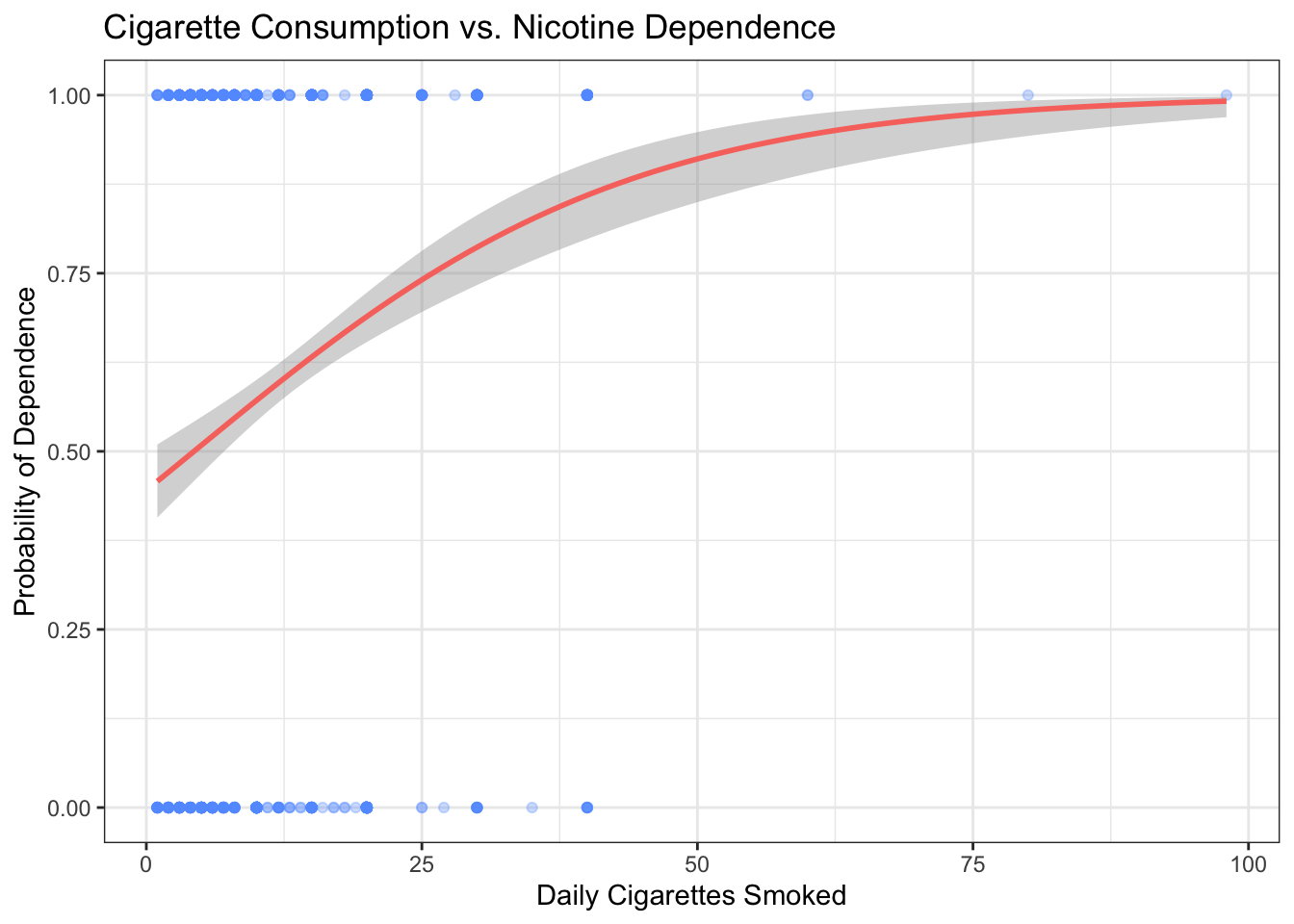
Figure 11.5: Logistic regression S-curve: the predicted probability of nicotine dependence increases with daily cigarette consumption, staying neatly within the 0–1 range.
The red curve is the same logistic model you just fit with glm(). Each blue dot is a person — stuck at the top (1 = dependent) or bottom (0 = not dependent). The curve shows how the probability of dependence climbs as cigarette consumption increases, without ever exceeding 1 or dipping below 0.
11.6.2 Example 2: Adding Depression as a Second Predictor
Now add depression to the model. This is like multiple regression (Chapter 10) — you are asking whether depression predicts nicotine dependence even after accounting for smoking quantity:
# Multiple logistic regression — two predictors
# ← REPLACE: binary_response ~ quant_var + cat_var,   data = your_df
logistic_multi <- glm(TobaccoDependence ~ DailyCigsSmoked + MajorDepression,
                       data = nesarc,
                       family = "binomial")           # binomial family = logistic
summary(logistic_multi)                                # view full output
##
## Call:
## glm(formula = TobaccoDependence ~ DailyCigsSmoked + MajorDepression,
## family = "binomial", data = nesarc)
##
## Coefficients:
## Estimate Std. Error z value Pr(>|z|)
## (Intercept) -0.548942 0.121392 -4.522 6.12e-06 ***
## DailyCigsSmoked 0.051841 0.008077 6.419 1.37e-10 ***
## MajorDepressionYes Depression 1.379662 0.153894 8.965 < 2e-16 ***
## ---
## Signif. codes: 0 '***' 0.001 '**' 0.01 '*' 0.05 '.' 0.1 ' ' 1
##
## (Dispersion parameter for binomial family taken to be 1)
##
## Null deviance: 1762.5 on 1314 degrees of freedom
## Residual deviance: 1620.8 on 1312 degrees of freedom
## (5 observations deleted due to missingness)
## AIC: 1626.8
##
## Number of Fisher Scoring iterations: 4# Odds ratios with 95% CI
tidy(logistic_multi, conf.int = TRUE, exponentiate = TRUE) %>% # exponentiated coefficients
select(term, estimate, conf.low, conf.high, p.value) %>% # keep key columns
rename(Term = term, `Odds Ratio` = estimate,
`95% CI Lower` = conf.low, `95% CI Upper` = conf.high,
`p-value` = p.value) %>%
knitr::kable(digits = 3,
caption = "Multiple Logistic Regression: Nicotine Dependence (Odds Ratios)")| Term | Odds Ratio | 95% CI Lower | 95% CI Upper | p-value |
|---|---|---|---|---|
| (Intercept) | 0.578 | 0.454 | 0.731 | 0 |
| DailyCigsSmoked | 1.053 | 1.037 | 1.070 | 0 |
| MajorDepressionYes Depression | 3.974 | 2.956 | 5.408 | 0 |
11.6.3 Side-by-Side Model Comparison
Use modelsummary() to compare the simple and multiple logistic regression models:
# Side-by-side comparison — simple vs. multiple logistic regression
# ← REPLACE: your_model1, your_model2
modelsummary(
  list("Simple" = logistic_simple, "Multiple" = logistic_multi),  # models to compare
  exponentiate = TRUE,                                             # show odds ratios
  statistic = "conf.int",                                          # show 95% CI
  conf_level = 0.95,                                               # confidence level
  stars = c('*' = .05, '**' = .01, '***' = .001),                 # significance stars
  title = "Logistic Regression Models: Nicotine Dependence"
)| Simple | Multiple | |
|---|---|---|
| * p < 0.05, ** p < 0.01, *** p < 0.001 | ||
| (Intercept) | 0.803 | 0.578*** |
| [0.643, 1.000] | [0.454, 0.731] | |
| DailyCigsSmoked | 1.052*** | 1.053*** |
| [1.036, 1.069] | [1.037, 1.070] | |
| MajorDepressionYes Depression | 3.974*** | |
| [2.956, 5.408] | ||
| Num.Obs. | 1315 | 1315 |
| AIC | 1718.5 | 1626.8 |
| BIC | 1728.8 | 1642.3 |
| Log.Lik. | -857.231 | -810.400 |
| F | 42.295 | 57.975 |
| RMSE | 0.48 | 0.46 |
This table lets your reader see at a glance whether adding depression changes the effect of daily cigarettes, and whether depression itself is a significant predictor.
11.6.4 Making a Prediction
One of the most useful things about logistic regression is predicting probabilities for specific profiles. Suppose you want to know: what is the predicted probability of nicotine dependence for a young adult smoker who smokes 10 cigarettes per day and has depression?
# Predict probability of nicotine dependence for a specific profile
# ← REPLACE: the values in the data frame below
new_profile <- data.frame(
  DailyCigsSmoked = 10,                     # 10 cigarettes per day
  MajorDepression = "Yes Depression"         # has depression
)

# predict() returns the predicted probability (type = "response")
predict(logistic_multi,                      # the fitted model
        newdata = new_profile,               # the profile to predict for
        type = "response")                   # output = probability (not log-odds)
## 1
## 0.793988# Predict for a second profile: same smoking, no depression
no_depression_profile <- data.frame(
DailyCigsSmoked = 10, # 10 cigarettes per day
MajorDepression = "No Depression" # no depression
)
predict(logistic_multi, # the fitted model
newdata = no_depression_profile, # the comparison profile
type = "response") # output = probability## 1
## 0.4923685The output is a probability between 0 and 1. A value of 0.65 means the model predicts a 65% chance that a young adult smoker with that profile has nicotine dependence.
11.6.5 Adding an Interaction in Logistic Regression
You can also test moderation within logistic regression. The concept is the same as in ANOVA — the * operator creates an interaction term:
# Logistic regression with interaction — tests moderation on a binary outcome
# Does the effect of daily cigarettes on dependence odds differ by depression?
# ← REPLACE: binary_response ~ quant_var * moderator_var,   data = your_df
logistic_interaction <- glm(TobaccoDependence ~ DailyCigsSmoked * MajorDepression,
                             data = nesarc,
                             family = "binomial")
summary(logistic_interaction)   # look at the interaction term p-value
##
## Call:
## glm(formula = TobaccoDependence ~ DailyCigsSmoked * MajorDepression,
## family = "binomial", data = nesarc)
##
## Coefficients:
## Estimate Std. Error z value
## (Intercept) -0.482676 0.128818 -3.747
## DailyCigsSmoked 0.046605 0.008738 5.334
## MajorDepressionYes Depression 1.000060 0.298838 3.347
## DailyCigsSmoked:MajorDepressionYes Depression 0.033242 0.023099 1.439
## Pr(>|z|)
## (Intercept) 0.000179 ***
## DailyCigsSmoked 9.62e-08 ***
## MajorDepressionYes Depression 0.000818 ***
## DailyCigsSmoked:MajorDepressionYes Depression 0.150125
## ---
## Signif. codes: 0 '***' 0.001 '**' 0.01 '*' 0.05 '.' 0.1 ' ' 1
##
## (Dispersion parameter for binomial family taken to be 1)
##
## Null deviance: 1762.5 on 1314 degrees of freedom
## Residual deviance: 1618.6 on 1311 degrees of freedom
## (5 observations deleted due to missingness)
## AIC: 1626.6
##
## Number of Fisher Scoring iterations: 5# Odds ratios for the interaction model
tidy(logistic_interaction, conf.int = TRUE, exponentiate = TRUE) %>%
select(term, estimate, conf.low, conf.high, p.value) %>%
rename(Term = term, `Odds Ratio` = estimate,
`95% CI Lower` = conf.low, `95% CI Upper` = conf.high,
`p-value` = p.value) %>%
knitr::kable(digits = 3,
caption = "Logistic Regression with Interaction (Odds Ratios)")| Term | Odds Ratio | 95% CI Lower | 95% CI Upper | p-value |
|---|---|---|---|---|
| (Intercept) | 0.617 | 0.478 | 0.793 | 0.000 |
| DailyCigsSmoked | 1.048 | 1.030 | 1.066 | 0.000 |
| MajorDepressionYes Depression | 2.718 | 1.516 | 4.898 | 0.001 |
| DailyCigsSmoked:MajorDepressionYes Depression | 1.034 | 0.990 | 1.083 | 0.150 |
The DailyCigsSmoked:MajorDepressionYes Depression row is the interaction. Its p-value tells you whether the effect of daily cigarettes on the odds of dependence differs by depression status — the same moderation concept you learned earlier, now applied to a binary outcome.
11.7 Interpretation: Logistic Regression
11.7.1 How to Read Logistic Regression Output — Quick Reference
| What to Find | Where It Is | What It Tells You |
|---|---|---|
| Estimate (log-odds) | Estimate column in summary() |
Direction and magnitude on the log-odds scale. Positive = increases odds; negative = decreases. |
| Odds Ratio | exp(coef(model)) or exponentiate = TRUE |
Multiplicative effect on odds per unit increase. OR > 1 increases odds; OR < 1 decreases. |
| p-value | Pr(>\|z\|) column |
If p < 0.05, the predictor is statistically significant. |
| 95% CI | confint() then exp(), or exponentiate = TRUE |
If the CI excludes 1.0, the predictor is significant. Width shows precision. |
| Null deviance | Top of summary() |
Model fit with no predictors (intercept only). |
| Residual deviance | Top of summary() |
Model fit with predictors. Lower = better fit. Compare to null deviance to gauge improvement. |
11.7.2 Writing Up Logistic Regression Results
For a single-predictor model:
A logistic regression revealed that daily cigarette consumption was significantly associated with nicotine dependence among young adult daily smokers (OR = X.XX, 95% CI [X.XX, X.XX], p < .001). For each additional cigarette smoked per day, the odds of nicotine dependence increased by approximately XX%.
To convert an odds ratio to a percentage change: \((OR - 1) \times 100\%\). For example, OR = 1.08 means an 8% increase in odds per unit of X.
For a multiple-predictor model:
After adjusting for depression status, daily cigarette consumption remained significantly associated with nicotine dependence (OR = X.XX, 95% CI [X.XX, X.XX], p < .001). Depression was [also / not] significantly associated with dependence after controlling for smoking quantity (OR = X.XX, p = .XXX).
11.7.3 Common Mistakes in Logistic Regression
- Interpreting odds ratios as risk ratios or probabilities. An OR of 2.0 does NOT mean the probability doubles. It means the odds double. If the baseline probability is 10% (odds = 0.11), doubling the odds gives odds of 0.22, which corresponds to a probability of about 18% — not 20%. The confusion gets worse for larger ORs.
How do you explain an odds ratio to a judge or classmate without sounding like a casino bookie? Try this: “For each additional cigarette per day, the odds of being dependent increase by about 8%. In plain terms: the more someone smokes, the more likely they are to be dependent — and the model tells us exactly how much that likelihood climbs.” If you need to avoid the word “odds” entirely, convert to a concrete example using predicted probabilities: “A young adult smoker at 5 cigarettes per day has about a 40% predicted chance of dependence. Someone at 20 per day has about an 80% chance.” Specific probabilities (from predict(..., type = "response")) are almost always more intuitive than odds ratios for a general audience.
Forgetting to exponentiate. The raw coefficients from
summary()are in log-odds units. A coefficient of 0.08 is NOT an 8% increase — you need to compute \(e^{0.08} \approx 1.083\), which gives an OR of 1.083 (an 8.3% increase in odds). Always useexp(coef())orexponentiate = TRUEintidy().Using logistic regression when the response has more than 2 categories. Logistic regression is designed for binary outcomes. If your response has three or more categories (e.g., “none,” “mild,” “severe”), you need multinomial logistic regression, which is beyond this book. Make sure your response variable is coded as 0/1 or a two-level factor.
Ignoring the confidence interval. A significant p-value with a very wide CI means your estimate is imprecise. The effect is real, but you cannot pin down its size with confidence. Always report the CI alongside the OR.
Over-interpreting non-significant predictors. If a predictor has p = 0.08, you cannot claim it has “no effect.” You can only say the evidence was not strong enough to reach statistical significance at the 0.05 level. The true effect might be real but small, or your sample might be too small to detect it.
Confusing odds with probability. Odds of 2.0 means 2:1 odds — the event is twice as likely to happen as not. That corresponds to a probability of \(2 / (2 + 1) = 0.667\), or 66.7%. It does NOT mean a 200% probability. If you need to report probabilities, use
predict(..., type = "response").
11.8 Reporting Checklist
When you write up a moderation analysis or logistic regression, include all six pieces:
11.9 A Brief Note on Confounding
You encountered confounding in Chapter 10 (Multiple Regression). It is worth revisiting here because logistic regression also handles it.
Confounding happens when a third variable explains the apparent relationship between X and Y. For example, suppose you find that daily cigarettes predict nicotine dependence. But what if depression causes both heavier smoking and higher dependence? In that case, part of the smoking-dependence link might be an artifact — depression is the real driver behind both.
Multiple logistic regression (adding depression as a second predictor) helps you address this. If the effect of daily cigarettes shrinks or disappears after adjusting for depression, that is evidence of confounding.
But remember: association does not imply causation. Even a well-specified logistic regression with multiple predictors cannot prove causation from observational data like the NESARC survey. You can rule out some confounders, but you can never rule them all out. This is why randomized experiments remain the gold standard for causal claims.
11.10 What Comes Next
You have now completed the full statistical toolkit. Look at what you can do:
- Describe data: frequency tables, summary statistics, graphs (Chapters 1–4)
- Test for differences: t-tests (Chapter 5), ANOVA (Chapter 6)
- Test for associations: Chi-Square (Chapter 7), Correlation (Chapter 8)
- Model relationships: linear regression (Chapter 9), multiple regression (Chapter 10)
- Handle complexity: moderation (Chapter 11), logistic regression for binary outcomes (Chapter 11)
Every statistical tool you have learned maps to a specific combination of variable types. Use the framework from Chapter 4 to choose the right tool:
| Response | Explanatory | Tool |
|---|---|---|
| Quantitative | Categorical (2 groups) | t-test (Ch 5) |
| Quantitative | Categorical (3+ groups) | ANOVA (Ch 6) |
| Categorical | Categorical | Chi-Square (Ch 7) |
| Quantitative | Quantitative | Correlation / Regression (Ch 8–9) |
| Quantitative | Multiple predictors | Multiple Regression (Ch 10) |
| Binary | Any | Logistic Regression (Ch 11) |
| Any | Any + Moderator | Interaction Term (Ch 11) |
Chapter 12 (Epilogue) will help you bring it all together. You will learn how to write up a complete analysis — from research question, through data management and exploratory analysis, through hypothesis testing, to a final conclusion. Everything you have learned in Chapters 1 through 11 comes together in one coherent write-up.