Chapter 10 Multiple Regression & Confounding
10.1 TL;DR: Multiple Regression
- Multiple regression extends simple regression by adding more than one predictor — you ask “what is the relationship between my response and this predictor, after accounting for those other variables?”
- A confounding variable is a third variable that is associated with both your explanatory variable and your response. If you ignore it, the simple regression coefficient can be biased — either inflated, deflated, or even reversed.
- “Controlling for” or “adjusting for” a variable means including it in the model so its influence is separated from the variable you care about. The resulting coefficient is the adjusted or partial effect.
- Add predictors with
+in the formula:lm(Y ~ X1 + X2 + X3, data = df). Categorical predictors with more than two levels are automatically expanded into dummy variables by R. - Compare models side-by-side with
modelsummary()to see how coefficients change when you add potential confounders. - \(R^2\) always increases when you add predictors (even useless ones). Use Adjusted \(R^2\) to compare models with different numbers of predictors.
# Load packages
library(ggplot2)         # for all graphing
library(dplyr)           # for filter(), rename(), select(), %>%
library(modelsummary)    # for professional regression tables

# Load the NESARC survey — ← REPLACE: your file path
NESARC <- read.csv("NESARC.csv")

# Build the subset we use throughout the book — ← REPLACE: your filter logic
nesarc <- NESARC %>%
  filter(
    S3AQ1A == 1,         # smoked 100+ cigarettes in lifetime
    S3AQ3B1 == 1,        # smoked in the past 12 months
    CHECK321 == 1,       # valid nicotine dependence data
    AGE <= 25             # young adults only
  ) %>%
  rename(
    Ethnicity          = ETHRACE2A,     # ← REPLACE: your variable names
    Age                = AGE,
    MajorDepression    = MAJORDEPLIFE,
    TobaccoDependence  = TAB12MDX,
    DailyCigsSmoked    = S3AQ3C1,
    Sex                = SEX
  ) %>%
  select(Ethnicity, Age, MajorDepression, TobaccoDependence, DailyCigsSmoked, Sex)

# Recode missing and label factors
nesarc$DailyCigsSmoked[nesarc$DailyCigsSmoked == 99] <- NA    # 99 = Unknown → NA
nesarc$MajorDepression <- factor(nesarc$MajorDepression,
  labels = c("No Depression", "Yes Depression"))               # ← REPLACE: your labels
nesarc$Sex <- factor(nesarc$Sex,
  labels = c("Female", "Male"))                                # ← REPLACE: your labels
nesarc$Ethnicity <- factor(nesarc$Ethnicity,
  labels = c("Caucasian", "African American", "Native American",
             "Asian", "Hispanic"))                              # ← REPLACE: your labels
# Model 1 — Simple regression: does depression predict cigarette consumption?
m1 <- lm(DailyCigsSmoked ~ MajorDepression, data = nesarc) # ← REPLACE: your vars
summary(m1) # Depression coefficient: look at p-value and estimate##
## Call:
## lm(formula = DailyCigsSmoked ~ MajorDepression, data = nesarc)
##
## Residuals:
## Min 1Q Median 3Q Max
## -12.904 -6.166 -3.166 6.834 84.834
##
## Coefficients:
## Estimate Std. Error t value Pr(>|t|)
## (Intercept) 13.1663 0.2790 47.188 <2e-16 ***
## MajorDepressionYes Depression 0.7374 0.5385 1.369 0.171
## ---
## Signif. codes: 0 '***' 0.001 '**' 0.01 '*' 0.05 '.' 0.1 ' ' 1
##
## Residual standard error: 8.654 on 1313 degrees of freedom
## (5 observations deleted due to missingness)
## Multiple R-squared: 0.001426, Adjusted R-squared: 0.0006653
## F-statistic: 1.875 on 1 and 1313 DF, p-value: 0.1712# Model 2 — Multiple regression: add Sex as a potential confounder
m2 <- lm(DailyCigsSmoked ~ MajorDepression + Sex, data = nesarc) # + adds predictor
summary(m2) # Compare the depression coefficient to Model 1 — did it change?##
## Call:
## lm(formula = DailyCigsSmoked ~ MajorDepression + Sex, data = nesarc)
##
## Residuals:
## Min 1Q Median 3Q Max
## -14.532 -5.772 -1.772 5.603 83.603
##
## Coefficients:
## Estimate Std. Error t value Pr(>|t|)
## (Intercept) 14.3967 0.3550 40.551 < 2e-16 ***
## MajorDepressionYes Depression 1.1352 0.5375 2.112 0.0349 *
## SexMale -2.6245 0.4765 -5.508 4.36e-08 ***
## ---
## Signif. codes: 0 '***' 0.001 '**' 0.01 '*' 0.05 '.' 0.1 ' ' 1
##
## Residual standard error: 8.559 on 1312 degrees of freedom
## (5 observations deleted due to missingness)
## Multiple R-squared: 0.024, Adjusted R-squared: 0.02251
## F-statistic: 16.13 on 2 and 1312 DF, p-value: 1.202e-07# Side-by-side comparison — ← REPLACE: list your models
modelsummary(list("Model 1" = m1, "Model 2" = m2),
estimate = "{estimate}{stars}",
statistic = "({std.error})",
gof_map = c("nobs", "r.squared", "adj.r.squared"),
title = "Comparing Simple and Multiple Regression")| Model 1 | Model 2 | |
|---|---|---|
| (Intercept) | 13.166*** | 14.397*** |
| (0.279) | (0.355) | |
| MajorDepressionYes Depression | 0.737 | 1.135* |
| (0.539) | (0.537) | |
| SexMale | -2.624*** | |
| (0.476) | ||
| Num.Obs. | 1315 | 1315 |
| R2 | 0.001 | 0.024 |
| R2 Adj. | 0.001 | 0.023 |
Key interpretation: In the simple regression (Model 1), depression was associated with about 0.74 more cigarettes per day, but this was not statistically significant (p = 0.17). After adding Sex to the model (Model 2), the depression coefficient increased to 1.14 and became statistically significant (p = 0.035). Controlling for Sex revealed a depression effect that was hidden in the simple regression. This is why multiple regression matters: the relationship you see between two variables can change dramatically when you account for other variables.
10.2 Deep Dive: Multiple Regression
10.2.1 Motivating Example
In Chapter 9, you learned to fit a straight line through a cloud of points — simple linear regression. You asked: “Can one variable predict another?” You used lm(Y ~ X) and interpreted the slope as “for every one-unit increase in X, Y changes by this much, on average.”
That works when your research question involves exactly two variables. But real research questions are rarely that simple. Consider this scenario:
Your research question is: “Does major depression predict higher daily cigarette consumption among young adult smokers?”
You run a simple regression:
\[\text{DailyCigsSmoked} = \beta_0 + \beta_1 \cdot \text{MajorDepression}\]
The output tells you that depressed smokers consume about 0.74 more cigarettes per day — but the p-value is 0.17. Not statistically significant. You conclude there is no relationship.
But then a classmate looks over your shoulder. “Wait,” she says. “What about sex? Females and males might smoke different amounts. And depression rates might differ between females and males too. If sex is related to both depression and smoking, your simple regression might be misleading.”
She is describing confounding. And she is right.
In this chapter, you will learn to answer questions like “Does depression predict smoking, after accounting for sex?” You will learn what confounding is, how to detect it, and how multiple regression lets you separate the effects of several variables at once. By the end, you will have a tool that moves your analyses from “what predicts Y?” to “what predicts Y, and does that relationship hold up when we consider other explanations?”
Let’s start by loading the data and building the same NESARC subset you have used throughout this book.
# Load the packages you need for this chapter
library(ggplot2)         # for all graphing
library(dplyr)           # for filter(), rename(), select(), %>%
library(modelsummary)    # for professional regression tables

# Load the NESARC survey (43,093 adults) — ← REPLACE: your file path
NESARC <- read.csv("NESARC.csv")

# Build the subset: young adult (≤25) daily smokers with valid nicotine data
# ← REPLACE: adapt filter, rename, factor labels to YOUR dataset
nesarc <- NESARC %>%
  filter(
    S3AQ1A == 1,         # smoked 100+ cigarettes in lifetime (1 = Yes)
    S3AQ3B1 == 1,        # smoked in the past 12 months (1 = Yes)
    CHECK321 == 1,       # valid nicotine dependence data (1 = valid)
    AGE <= 25             # young adults only (≤ 25 years old)
  ) %>%
  rename(
    Ethnicity          = ETHRACE2A,     # ← REPLACE: rename to meaningful names
    Age                = AGE,           # age in years
    MajorDepression    = MAJORDEPLIFE,  # lifetime depression diagnosis (0/1)
    TobaccoDependence  = TAB12MDX,      # tobacco dependence, past 12 months (0/1)
    DailyCigsSmoked    = S3AQ3C1,       # usual cigarettes smoked per day
    Sex                = SEX            # sex (1=Female, 2=Male)
  ) %>%
  select(Ethnicity, Age, MajorDepression, TobaccoDependence, DailyCigsSmoked, Sex)

# Recode missing values — 99 means "Unknown" in the NESARC code book
nesarc$DailyCigsSmoked[nesarc$DailyCigsSmoked == 99] <- NA    # ← REPLACE: your NA codes

# Convert numeric codes into readable labels (factors)
nesarc$MajorDepression <- factor(nesarc$MajorDepression,
  labels = c("No Depression", "Yes Depression"))               # ← REPLACE: your labels
nesarc$Sex <- factor(nesarc$Sex,
  labels = c("Female", "Male"))                                # ← REPLACE: your labels
nesarc$Ethnicity <- factor(nesarc$Ethnicity,
  labels = c("Caucasian", "African American", "Native American",
             "Asian", "Hispanic"))                              # ← REPLACE: your labels
What just happened? Same data management recipe from Chapter 3: load, filter, rename, recode, label. The nesarc data frame has 1,320 observations of young adult daily smokers with six clean, labeled variables. You will use this single dataset for every analysis in this chapter.
10.2.1.1 Step 1: The Simple Regression
Let’s begin by running the simple regression — the kind you learned in Chapter 9. We predict daily cigarette consumption from depression status alone:
# Model 1 — Simple linear regression: does depression predict cigarette consumption?
# ← REPLACE: response ~ predictor,   data = your_df
m1 <- lm(DailyCigsSmoked ~ MajorDepression,    # formula: response ~ predictor
         data = nesarc)                         # the data frame
summary(m1)
##
## Call:
## lm(formula = DailyCigsSmoked ~ MajorDepression, data = nesarc)
##
## Residuals:
## Min 1Q Median 3Q Max
## -12.904 -6.166 -3.166 6.834 84.834
##
## Coefficients:
## Estimate Std. Error t value Pr(>|t|)
## (Intercept) 13.1663 0.2790 47.188 <2e-16 ***
## MajorDepressionYes Depression 0.7374 0.5385 1.369 0.171
## ---
## Signif. codes: 0 '***' 0.001 '**' 0.01 '*' 0.05 '.' 0.1 ' ' 1
##
## Residual standard error: 8.654 on 1313 degrees of freedom
## (5 observations deleted due to missingness)
## Multiple R-squared: 0.001426, Adjusted R-squared: 0.0006653
## F-statistic: 1.875 on 1 and 1313 DF, p-value: 0.1712Let’s read this output. The (Intercept) of 13.17 is the mean cigarettes per day for the reference group: people without depression. The MajorDepressionYes Depression coefficient of 0.74 means that, on average, people with depression smoke 0.74 more cigarettes per day than those without.
The p-value for the depression coefficient is 0.17 — above the 0.05 threshold. If you stopped here, you would write: “Depression was not significantly associated with daily cigarette consumption (b = 0.74, p = 0.17).”
The \(R^2\) is 0.0014 — depression alone explains only 0.14% of the variation in cigarette consumption. In other words, knowing someone’s depression status tells you almost nothing about how much they smoke.
But is that the whole story? Let’s look at the data more carefully.
10.2.1.2 Step 2: Is Something Missing?
Before you accept the simple regression result, think about what else might be going on. Here are two facts about the young adult daily smokers in the NESARC:
# Fact 1: Sex is associated with cigarette consumption — females smoke more in this subset
tapply(nesarc$DailyCigsSmoked, nesarc$Sex, mean, na.rm = TRUE)  # group means
## Female Male
## 14.63256 12.14328# Fact 2: Depression rates differ by sex — more females have depression
# ← REPLACE: your potential confounder
prop.table(table(nesarc$Sex, nesarc$MajorDepression), margin = 1) %>% round(3)##
## No Depression Yes Depression
## Female 0.793 0.207
## Male 0.672 0.328In this sample, females smoke about 2.6 more cigarettes per day than males — a substantial difference. And females have a higher rate of depression (about 27%) compared to males (about 16%). Sex is associated with both the predictor (depression) and the response (cigarette consumption).
This is the textbook setup for confounding:
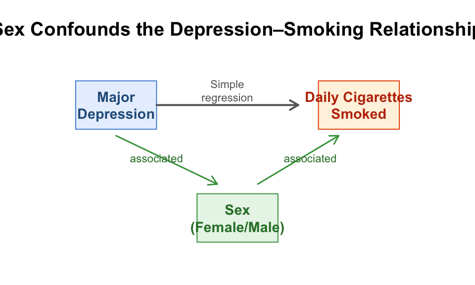
Figure 10.1: Sex is associated with both depression and cigarette consumption. The simple regression may confuse the effect of sex with the effect of depression.
When a third variable is associated with both your predictor and your response, the simple regression coefficient is a mixture of the true effects. It does not separate the influence of depression from the influence of sex — it lumps them together. The result can be misleading: the depression effect might be overestimated, underestimated, or even hidden entirely.
The solution is to control for the potential confounder by adding it to the regression model. This is multiple regression.
10.2.2 Theory
10.2.2.1 What Is Confounding?
A confounding variable (also called a lurking variable or confounder) is a variable that is associated with both the explanatory variable and the response variable, and that can create a false impression of a relationship — or mask a real one.
The classic example from everyday life: Ice cream sales and drowning deaths are positively correlated. As ice cream sales go up, so do drownings. Does ice cream cause drowning? Of course not. The confounding variable is temperature: hot weather causes people to buy more ice cream AND to go swimming more often. If you only look at ice cream sales and drownings, you see a correlation. If you control for temperature, the correlation disappears — ice cream adds no predictive power once you know the temperature.
The same logic applies to your research. When you find an association between two variables, always ask: “Is there a third variable that could explain this?”
Here are some potential confounders in the NESARC data:
| Explanatory Variable | Response Variable | Potential Confounder | Why? |
|---|---|---|---|
| Major Depression | Daily Cigarettes | Sex | Females smoke more (in this sample) AND have higher depression rates |
| Major Depression | Daily Cigarettes | Age | Older young adults may smoke more, and depression rates might vary with age |
| Tobacco Dependence | Daily Cigarettes | Major Depression | Depression might cause both dependence and heavier smoking |
10.2.2.2 How Multiple Regression Controls for Confounding
Simple regression answers: “What is the relationship between X and Y?”
Multiple regression answers: “What is the relationship between X and Y, holding other variables constant?”
When you fit lm(DailyCigsSmoked ~ MajorDepression + Sex), R estimates two coefficients simultaneously:
The coefficient for MajorDepression is the average difference in cigarette consumption between depressed and non-depressed people of the same sex. It is the effect of depression after removing the variation that comes from sex differences.
The coefficient for Sex is the average difference between males and females with the same depression status. It is the effect of sex after removing the variation that comes from depression differences.
These are called partial regression coefficients. Each one tells you the effect of that variable while holding all other variables in the model constant. The phrase “holding constant” or “controlling for” means: we compare people who are the same on the other variables and differ only on the variable of interest.
How does R actually “hold constant” behind the scenes — does it pretend everyone is the same gender? No. Mathematically, R performs a two-step cleanup: first, it regresses depression on sex and extracts the residuals (what is left of depression after removing everything sex can explain). Then it does the same for smoking — regresses smoking on sex and extracts the residuals (what is left of smoking after removing sex). Finally, it computes the relationship between these two sets of residuals. What remains is the pure depression–smoking relationship, with the influence of sex stripped away. This is why coefficients change when you add confounders: you are isolating different parts of the relationship each time.
In the confounding diagram above, multiple regression “blocks” the paths from Sex to both Depression and Smoking, isolating the direct path from Depression to Smoking.
10.2.2.3 The Multiple Regression Equation
The general form of a multiple regression model with \(k\) predictors is:
\[Y = \beta_0 + \beta_1 X_1 + \beta_2 X_2 + \cdots + \beta_k X_k + \varepsilon\]
- \(Y\) is the response variable (quantitative)
- \(X_1, X_2, \ldots, X_k\) are the predictor variables (quantitative or categorical)
- \(\beta_0\) is the intercept — the predicted value when all predictors equal zero (or their reference level)
- \(\beta_1\) is the partial slope for \(X_1\) — the average change in \(Y\) for a one-unit increase in \(X_1\), holding \(X_2, \ldots, X_k\) constant
- \(\beta_2\) is the partial slope for \(X_2\) — the average change in \(Y\) for a one-unit increase in \(X_2\), holding \(X_1, X_3, \ldots, X_k\) constant
- \(\varepsilon\) is the error term — the difference between the predicted and actual values
Each \(\beta\) is estimated from the data, just like in simple regression. The difference is that now each estimate accounts for the presence of the other predictors. The R syntax is exactly what you would guess:
The + sign means “add another predictor.” It does not mean addition in the mathematical sense — it means “include this variable in the model.”
10.2.2.4 Categorical Predictors in Regression
In Model 2 (DailyCigsSmoked ~ MajorDepression + Sex), both predictors are categorical with two levels. R handles categorical predictors automatically through dummy coding: it creates a binary (0/1) variable for each non-reference category.
For Sex with levels “Female” and “Male”:
- R picks “Female” as the reference category (first alphabetically)
- It creates a dummy variable: SexMale = 1 if Male, 0 if Female
- The SexMale coefficient means: “the average difference between males and females, holding other variables constant”
When a categorical predictor has more than two levels — like Ethnicity with five categories — R creates one dummy variable for each non-reference category:
| Ethnicity (original) | African American (1=yes) | Native American (1=yes) | Asian (1=yes) | Hispanic (1=yes) |
|---|---|---|---|---|
| Caucasian | 0 | 0 | 0 | 0 |
| African American | 1 | 0 | 0 | 0 |
| Native American | 0 | 1 | 0 | 0 |
| Asian | 0 | 0 | 1 | 0 |
| Hispanic | 0 | 0 | 0 | 1 |
You do not need to create these dummy variables yourself — R does it automatically when you include a factor in lm(). But understanding what happens behind the scenes helps you interpret the output: each ethnicity coefficient compares that group to the reference group (Caucasian), holding other variables constant.
10.2.2.5 Evaluating the Model: \(R^2\) and Adjusted \(R^2\)
In simple regression, \(R^2\) tells you the proportion of variation in \(Y\) explained by the single predictor. In multiple regression, \(R^2\) tells you the proportion of variation in \(Y\) explained by all the predictors together.
Important: \(R^2\) always increases (or at least never decreases) when you add more predictors to a model — even if those predictors are completely random noise. This is because \(R^2\) rewards models for fitting the data more closely, and more predictors always allow a closer fit, even if only by accident.
To compare models with different numbers of predictors fairly, use Adjusted \(R^2\):
\[\text{Adjusted } R^2 = 1 - \frac{(1 - R^2)(n - 1)}{n - k - 1}\]
where \(n\) is the sample size and \(k\) is the number of predictors. Adjusted \(R^2\) applies a penalty for each additional predictor. It only increases if the new predictor adds enough explanatory power to justify its inclusion.
When comparing models, look at both — \(R^2\) for the raw explanatory power, and Adjusted \(R^2\) to decide whether adding a predictor was truly worthwhile.
Can Adjusted \(R^2\) actually go down? Yes — and that is exactly the behavior you want. If you add a predictor that contributes essentially no explanatory power, the penalty outweighs the tiny gain in raw \(R^2\), and Adjusted \(R^2\) drops. For models that fit worse than simply guessing the mean of Y, Adjusted \(R^2\) can even become slightly negative — a clear signal that your model is not working. A decrease in Adjusted \(R^2\) tells you the new variable is not pulling its weight and probably should not be in the model. This built-in honesty is why Adjusted \(R^2\) is preferred over raw \(R^2\) for model comparison.
10.2.3 Code
Now let’s apply these concepts to the NESARC data. We will build four models, adding one predictor at a time, and compare the coefficients at each step. The question we are investigating:
“Does major depression predict daily cigarette consumption, after accounting for sex, age, and ethnicity?”
10.2.3.1 Model 1: Simple Regression (Depression Only)
# Model 1 — Simple regression: just depression as a predictor
# ← REPLACE: response ~ predictor
m1 <- lm(DailyCigsSmoked ~ MajorDepression, data = nesarc)
summary(m1)
##
## Call:
## lm(formula = DailyCigsSmoked ~ MajorDepression, data = nesarc)
##
## Residuals:
## Min 1Q Median 3Q Max
## -12.904 -6.166 -3.166 6.834 84.834
##
## Coefficients:
## Estimate Std. Error t value Pr(>|t|)
## (Intercept) 13.1663 0.2790 47.188 <2e-16 ***
## MajorDepressionYes Depression 0.7374 0.5385 1.369 0.171
## ---
## Signif. codes: 0 '***' 0.001 '**' 0.01 '*' 0.05 '.' 0.1 ' ' 1
##
## Residual standard error: 8.654 on 1313 degrees of freedom
## (5 observations deleted due to missingness)
## Multiple R-squared: 0.001426, Adjusted R-squared: 0.0006653
## F-statistic: 1.875 on 1 and 1313 DF, p-value: 0.1712How to read this output:
- Intercept (13.17): The predicted mean cigarettes per day for a person in the reference category — “No Depression.” A non-depressed young adult daily smoker smokes about 13.2 cigarettes per day, on average.
- MajorDepressionYes Depression (0.74): Depressed smokers consume about 0.74 more cigarettes per day than non-depressed smokers. The p-value is 0.17 — not statistically significant at the 0.05 level.
- \(R^2\) = 0.0014: Depression explains only 0.14% of the variation in cigarette consumption. This model fits the data very poorly.
If we stopped here, the conclusion would be: “No significant relationship between depression and smoking.” But we know (from our exploration above) that Sex is associated with both — let’s add it to the model.
10.2.3.2 Model 2: Add Sex — Control for a Potential Confounder
# Model 2 — Multiple regression: add Sex as a potential confounder
# ← REPLACE: response ~ predictor + confounder1
m2 <- lm(DailyCigsSmoked ~ MajorDepression + Sex, data = nesarc)
summary(m2)
##
## Call:
## lm(formula = DailyCigsSmoked ~ MajorDepression + Sex, data = nesarc)
##
## Residuals:
## Min 1Q Median 3Q Max
## -14.532 -5.772 -1.772 5.603 83.603
##
## Coefficients:
## Estimate Std. Error t value Pr(>|t|)
## (Intercept) 14.3967 0.3550 40.551 < 2e-16 ***
## MajorDepressionYes Depression 1.1352 0.5375 2.112 0.0349 *
## SexMale -2.6245 0.4765 -5.508 4.36e-08 ***
## ---
## Signif. codes: 0 '***' 0.001 '**' 0.01 '*' 0.05 '.' 0.1 ' ' 1
##
## Residual standard error: 8.559 on 1312 degrees of freedom
## (5 observations deleted due to missingness)
## Multiple R-squared: 0.024, Adjusted R-squared: 0.02251
## F-statistic: 16.13 on 2 and 1312 DF, p-value: 1.202e-07Now compare Model 2 to Model 1. Look at the depression coefficient:
| Model | Depression Coefficient | p-value | \(R^2\) |
|---|---|---|---|
| Model 1 (depression alone) | 0.74 | 0.17 | 0.0014 |
| Model 2 (+ Sex) | 1.14 | 0.035 | 0.0240 |
Three things happened when we added Sex:
The depression coefficient increased — from 0.74 to 1.14. That is a 54% increase. In Model 1, the depression coefficient was a mixture of the true depression effect and the sex effect. By adding Sex, we “untangled” them. The adjusted coefficient (1.14) is the estimated effect of depression for people of the same sex. This is closer to the true relationship.
The depression p-value dropped below 0.05 — from 0.17 to 0.035. The effect is now statistically significant. This is a case of suppression: the simple regression masked a real relationship because it could not separate depression from sex. The multiple regression revealed it.
\(R^2\) increased — from 0.0014 to 0.024. Sex adds meaningful explanatory power. The model now explains 2.4% of the variation, up from 0.14%.
The Sex coefficient (-2.62): This means that, holding depression status constant, males smoke about 2.6 fewer cigarettes per day than females in this sample of young adult daily smokers. The negative sign might surprise you (we often assume males smoke more), but in this specific subset — young adults who already smoke daily — females consume more cigarettes on average. Always let the data speak. The p-value is extremely small (p < 0.001), so this difference is clearly not due to chance.
Key insight: The simple regression asked “what is the relationship between depression and smoking?” and got a weak, non-significant answer. The multiple regression asked “what is the relationship between depression and smoking, after accounting for sex?” and got a stronger, significant answer. This is why you should always consider potential confounders — they can hide real relationships as easily as they can create false ones.
10.2.3.3 Model 3: Add Age — Another Potential Confounder
People’s smoking habits often change with age. Let’s add Age as a quantitative predictor:
# Model 3 — Add a quantitative predictor (Age)
# ← REPLACE: add another predictor with +
m3 <- lm(DailyCigsSmoked ~ MajorDepression + Sex + Age, data = nesarc)
summary(m3)
##
## Call:
## lm(formula = DailyCigsSmoked ~ MajorDepression + Sex + Age, data = nesarc)
##
## Residuals:
## Min 1Q Median 3Q Max
## -14.304 -5.774 -1.973 5.497 84.022
##
## Coefficients:
## Estimate Std. Error t value Pr(>|t|)
## (Intercept) 10.6534 2.3430 4.547 5.95e-06 ***
## MajorDepressionYes Depression 1.1506 0.5372 2.142 0.0324 *
## SexMale -2.7046 0.4787 -5.649 1.97e-08 ***
## Age 0.1750 0.1083 1.616 0.1063
## ---
## Signif. codes: 0 '***' 0.001 '**' 0.01 '*' 0.05 '.' 0.1 ' ' 1
##
## Residual standard error: 8.554 on 1311 degrees of freedom
## (5 observations deleted due to missingness)
## Multiple R-squared: 0.02594, Adjusted R-squared: 0.02371
## F-statistic: 11.64 on 3 and 1311 DF, p-value: 1.579e-07Age is quantitative (18–25 years in this subset), so it enters the model directly — R does not create dummy variables for it. The Age coefficient of 0.175 means: for every additional year of age, daily cigarette consumption increases by about 0.175 cigarettes, holding depression and sex constant. Over the 7-year age range in our sample (18 to 25), this translates to about 1.2 more cigarettes per day for a 25-year-old compared to an 18-year-old.
The depression and sex coefficients remained nearly unchanged (1.15 and -2.70, vs. 1.14 and -2.62 in Model 2), which tells us Age is not a strong confounder for the depression–smoking relationship. Adding Age increased \(R^2\) only slightly (from 0.0240 to 0.0259).
10.2.3.4 Model 4: Add Ethnicity — A Multi-Level Categorical Predictor
Ethnicity is a categorical variable with five levels. Let’s add it and see how R handles it:
# Model 4 — Add a multi-level categorical predictor (Ethnicity)
# ← REPLACE: add your categorical predictor
m4 <- lm(DailyCigsSmoked ~ MajorDepression + Sex + Age + Ethnicity, data = nesarc)
summary(m4)
##
## Call:
## lm(formula = DailyCigsSmoked ~ MajorDepression + Sex + Age +
## Ethnicity, data = nesarc)
##
## Residuals:
## Min 1Q Median 3Q Max
## -15.810 -5.760 -1.429 4.100 86.933
##
## Coefficients:
## Estimate Std. Error t value Pr(>|t|)
## (Intercept) 12.3753 2.2714 5.448 6.07e-08 ***
## MajorDepressionYes Depression 1.0283 0.5207 1.975 0.0485 *
## SexMale -2.8750 0.4634 -6.204 7.38e-10 ***
## Age 0.1762 0.1046 1.684 0.0923 .
## EthnicityAfrican American -4.6567 0.6950 -6.701 3.08e-11 ***
## EthnicityNative American -1.5653 1.5395 -1.017 0.3094
## EthnicityAsian -5.6992 1.2397 -4.597 4.70e-06 ***
## EthnicityHispanic -4.6683 0.6240 -7.481 1.35e-13 ***
## ---
## Signif. codes: 0 '***' 0.001 '**' 0.01 '*' 0.05 '.' 0.1 ' ' 1
##
## Residual standard error: 8.266 on 1307 degrees of freedom
## (5 observations deleted due to missingness)
## Multiple R-squared: 0.09314, Adjusted R-squared: 0.08828
## F-statistic: 19.18 on 7 and 1307 DF, p-value: < 2.2e-16Look at the ethnicity coefficients. R created four dummy variables behind the scenes (as shown in the table in the Theory section). Each coefficient compares that ethnic group to the reference group (Caucasian):
- African American: -4.66 fewer cigarettes per day than Caucasian (p < 0.001)
- Native American: -1.57 fewer (p = 0.31, not significant)
- Asian: -5.70 fewer (p < 0.001)
- Hispanic: -4.67 fewer (p < 0.001)
All coefficients are negative, meaning every non-Caucasian group in this sample smokes fewer cigarettes per day on average than Caucasians, holding depression, sex, and age constant. Some of these differences are large — over 4 cigarettes per day — and highly significant.
Why is Caucasian the reference group — and why is it invisible in the output? R chooses the first level alphabetically as the reference by default, and the reference group’s coefficient is always zero (it is the baseline everything else is compared to). You can change the reference category using relevel(): nesarc$Ethnicity <- relevel(nesarc$Ethnicity, ref = "Hispanic") would make Hispanic the new baseline, and all coefficients would then compare each group to Hispanic instead. If you reorder factor levels with factor(..., levels = c("Hispanic", "Caucasian", ...)), R uses whichever group appears first as the reference. Choose a reference group that makes substantive sense for your research question — often the largest group or the one you want to compare others against.
\(R^2\) jumped from 0.026 to 0.093 — ethnicity explains substantially more variation in cigarette consumption than depression, sex, or age. The model now explains about 9.3% of the variation in daily cigarette consumption, a major improvement over the 0.14% we started with.
The depression coefficient dropped slightly (from 1.15 to 1.03) and its p-value increased (from 0.032 to 0.048), still significant but closer to the threshold. This suggests that ethnicity partly — but not fully — accounts for the depression–smoking relationship.
10.2.3.5 Comparing All Four Models Side-by-Side
The most powerful way to see how coefficients change as you add predictors is to put all four models in one table:
# Side-by-side comparison of all four models — ← REPLACE: list your models
library(modelsummary)
modelsummary(list("(1) Depression" = m1,
                  "(2) + Sex"      = m2,
                  "(3) + Age"      = m3,
                  "(4) + Ethnicity"= m4),
             estimate = "{estimate}{stars}",
             statistic = "({std.error})",
             stars = TRUE,
             gof_map = c("nobs", "r.squared", "adj.r.squared"),
title = "Multiple Regression: Predicting Daily Cigarette Consumption")| (1) Depression | (2) + Sex | (3) + Age | (4) + Ethnicity | |
|---|---|---|---|---|
| (Intercept) | 13.166*** | 14.397*** | 10.653*** | 12.375*** |
| (0.279) | (0.355) | (2.343) | (2.271) | |
| MajorDepressionYes Depression | 0.737 | 1.135* | 1.151* | 1.028* |
| (0.539) | (0.537) | (0.537) | (0.521) | |
| SexMale | -2.624*** | -2.705*** | -2.875*** | |
| (0.476) | (0.479) | (0.463) | ||
| Age | 0.175 | 0.176+ | ||
| (0.108) | (0.105) | |||
| EthnicityAfrican American | -4.657*** | |||
| (0.695) | ||||
| EthnicityNative American | -1.565 | |||
| (1.540) | ||||
| EthnicityAsian | -5.699*** | |||
| (1.240) | ||||
| EthnicityHispanic | -4.668*** | |||
| (0.624) | ||||
| Num.Obs. | 1315 | 1315 | 1315 | 1315 |
| R2 | 0.001 | 0.024 | 0.026 | 0.093 |
| R2 Adj. | 0.001 | 0.023 | 0.024 | 0.088 |
Read this table from left to right. Each column is a model. Each row is a coefficient. The stars (* = p < 0.05, ** = p < 0.01, *** = p < 0.001) indicate statistical significance.
Why the list() wrapper around the models? modelsummary() expects all models bundled into a single object — a list — rather than passed as separate arguments. The syntax list("Model 1" = m1, "Model 2" = m2) creates a named list where the names (“Model 1”, “Model 2”) become the column headers in the output table. If you wrote modelsummary(m1, m2) without list(), R would misinterpret m2 as a second function argument and likely produce an error. The list() wrapper tells R “these models are a set — display them side by side.”
What to notice:
The depression coefficient drifted across models — from 0.74 (not significant) in Model 1 to 1.14 (significant) when Sex was added. It stabilized around 1.0–1.15 in Models 2–4. This is the “confounding check”: if adding a variable causes a large change in your coefficient of interest, that variable was confounding the simple relationship.
Some predictors are consistently significant (Sex, several Ethnicity categories) — you can be confident these are real effects.
\(R^2\) and Adjusted \(R^2\) track together — Adjusted \(R^2\) increased with each added predictor, confirming that all four variables contribute meaningful information above and beyond what was already in the model.
The intercept changes across models — from 13.2 (Model 1) to 12.4 (Model 4). The intercept always represents the predicted value when all predictors are zero (or at their reference level), so it changes as the reference conditions change.
10.2.3.6 Visualizing Multiple Regression
You cannot graph a four-dimensional relationship on a flat page, but you can use facet_grid() to show how the depression–smoking relationship looks within each sex:
# Visualize the confounding: depression vs. cigarettes, split by sex
# ← REPLACE: x = predictor, y = response, facet = confounder
ggplot(data = nesarc, aes(x = MajorDepression, y = DailyCigsSmoked)) +
  geom_boxplot(fill = "#619CFF") +                            # boxplot per group
  theme_bw() +
  labs(x = "", y = "Daily Cigarettes Smoked",
       title = "Depression and Smoking, by Sex") +
  facet_grid(. ~ Sex)                                          # split panels by sex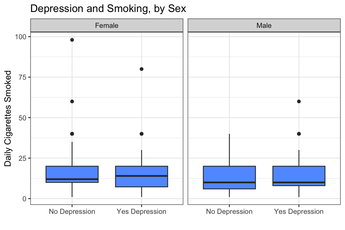
The boxplots show the raw data. Notice that females (left panel) smoke more cigarettes on average than males (right panel) — the boxes sit higher. Within each sex, the “Yes Depression” box is slightly higher than the “No Depression” box — that is the depression effect, holding sex constant. The pattern is subtle, but the regression detected it.
What if your final model has five or more predictors? You cannot graph a 5-dimensional relationship on a flat page, and you should not try. Instead, create one or two focused visualizations of your most important finding — faceting by a key confounder (like the Sex example above) is a powerful and clean pattern. Let the modelsummary() table handle the rest. A well-organized coefficient table alongside one targeted graph tells a far more compelling story than a cluttered attempt to show everything at once. In published scientific papers, the regression table often carries more evidentiary weight than the figures — it is where the formal hypothesis tests live.
10.2.4 Interpretation
10.2.4.1 How to Read Multiple Regression Output
When you see summary() output for a multiple regression, focus on these elements:
| Output Element | What It Tells You | Where to Look |
|---|---|---|
| Coefficient estimate | The average change in Y for a one-unit increase in X, holding other predictors constant. For categorical predictors, the difference from the reference group. | The Estimate column |
| Standard error | The uncertainty around the estimate. Larger standard error = less precise estimate. | The Std. Error column |
| t-value | The estimate divided by its standard error. Larger absolute values = stronger evidence against the null (no effect). | The t value column |
| p-value | The probability of seeing a t-value this extreme if the true coefficient were zero. p < 0.05 → significant. | The Pr(>|t|) column |
| \(R^2\) | Proportion of variation in Y explained by all predictors together. Higher = better fit. | Bottom of summary() |
| Adjusted \(R^2\) | \(R^2\) penalized for the number of predictors. Use this to compare models. | Bottom of summary() |
| F-statistic | Tests whether the model as a whole explains more variation than a model with no predictors. Small p-value → at least one predictor is useful. | Bottom of summary() |
Golden rule for interpretation: The coefficient for any predictor is the effect of that predictor assuming all other predictors in the model are held constant. If you leave a variable out, its effect gets mixed into the coefficients of whatever predictors it is correlated with.
10.2.4.2 Before vs. After Comparison
The most important skill in this chapter is comparing coefficients across models to detect confounding. Here is the checklist:
- Fit a simple regression with your predictor of interest and your response.
- Identify potential confounders — variables that might be associated with both the predictor and the response. Use domain knowledge and exploratory analysis.
- Add each potential confounder one at a time and observe how the coefficient of interest changes.
- A large change (>10–20% in the coefficient) suggests confounding. The adjusted coefficient (from the model that includes the confounder) is the more trustworthy estimate.
- Report the adjusted coefficient: “After controlling for [confounders], [predictor] was [significantly/not significantly] associated with [response].”
In our example:
- Simple regression (Model 1): Depression coefficient = 0.74 (p = 0.17, not significant)
- After controlling for Sex (Model 2): Depression coefficient = 1.14 (p = 0.035, significant)
The coefficient changed by over 50%, and a null finding became significant. This is a textbook case of why you must check for confounding.
10.2.4.3 Writing Up Your Results
When you report a multiple regression in a paper or poster (Chapter 12, Appendix B), include:
- The predictors in the model
- The key coefficient(s) of interest
- Whether the effect was statistically significant
- What variables were controlled for
- The model fit (\(R^2\) or Adjusted \(R^2\))
Here is the standard format:
A multiple regression was conducted to predict daily cigarette consumption from major depression, sex, age, and ethnicity (Table 1). After controlling for sex, age, and ethnicity, major depression was significantly associated with higher daily cigarette consumption (b = 1.03, SE = 0.52, p = 0.048). On average, young adult daily smokers with depression smoked about one more cigarette per day than those without depression, holding other factors constant. The full model explained 9.3% of the variance in daily cigarette consumption (Adjusted \(R^2\) = 0.087, F(7, 1265) = 18.55, p < 0.001). Sex and ethnicity were also significant predictors, with males smoking fewer cigarettes than females, and all non-Caucasian ethnic groups smoking fewer cigarettes than Caucasians, on average.
Notice the phrase “After controlling for…” — this signals to your reader that the reported coefficient has been adjusted for the other variables in the model. Good write-ups always specify what was controlled for.
10.2.4.4 Common Mistakes Students Make
- Ignoring potential confounders. The most common error is running a simple regression and stopping there. Always ask: “What else could explain this relationship?” If you cannot think of any confounders, ask someone else to look at your analysis. Fresh eyes often spot what you missed.
How many confounders do you need? You will never catch them all — that is the honest truth of observational research. An unmeasured variable could always exist. The goal in this book is not to eliminate every possible source of confounding (impossible) but to address the most obvious and well-documented ones suggested by your domain knowledge. If you control for the 3–4 most plausible alternative explanations and your result holds up, you have a defensible analysis. In your final report, acknowledge the limitation: “This analysis controlled for sex, age, and ethnicity. Other unmeasured variables may also influence the relationship.” Honesty about limitations is a scientific strength, not a weakness.
Adding too many predictors. Every predictor you add consumes a degree of freedom. With a small sample (say, n = 50), adding 10 predictors will overfit the model — it will describe your particular sample beautifully but predict new data poorly. A rough rule of thumb: aim for at least 10–20 observations per predictor.
Confusing correlation among predictors with a problem. Predictors are often correlated with each other — that is why confounding exists. Moderate correlation is fine; multiple regression is designed to handle it. Only extreme correlation (multicollinearity) causes problems, making standard errors blow up and coefficients unstable.
Over-interpreting small changes in coefficients. A coefficient changing from 0.74 to 0.77 is probably just noise. A change from 0.74 to 1.14 (or from significant to non-significant) is worth investigating. Focus on substantial changes, not tiny fluctuations.
Forgetting to check the sign. If adding a confounder flips your coefficient from positive to negative (or vice versa), that is a major red flag. This is called Simpson’s paradox and demands careful investigation.
Reporting unadjusted coefficients when confounders are present. If you know Sex confounds the depression–smoking relationship, do not report the simple regression coefficient. Report the adjusted coefficient from the model that includes Sex. The unadjusted coefficient is misleading.
Using \(R^2\) instead of Adjusted \(R^2\) to compare models. \(R^2\) always increases with more predictors. Adjusted \(R^2\) tells you whether the added predictor was worth its cost in complexity. Always report Adjusted \(R^2\) when comparing models.
Treating “controlling for” as “making causal.” Adding confounders to a regression does not magically turn an observational study into an experiment. It reduces bias from the confounders you can measure, but unmeasured confounders remain. Be humble in your causal claims, especially with observational data like surveys.
10.2.4.5 What Comes Next
You have now learned to build models with multiple predictors, check for confounding, and interpret partial regression coefficients. You can ask not just “does X predict Y?” but “does X predict Y, even after accounting for Z?”
But all of the models in this chapter assumed that the relationship between each predictor and the response is the same for everyone — that the effect of depression on smoking is the same for females and males, that the effect of age does not depend on ethnicity. What if those assumptions are wrong?
In Chapter 11 (Moderation & Extensions), you will learn about interactions — what happens when the effect of one predictor depends on the level of another predictor. For example, does depression affect smoking differently for females than for males? Does the relationship between age and cigarette consumption change across ethnic groups? Interaction terms let you ask and answer these questions.