Chapter 7 Chi-Square — Testing Associations

7.1 TL;DR: Chi-Square

The chi-square test of independence tests whether two categorical variables (C→C) are associated in the population — or whether the pattern you see could be sampling noise.
$H_0$: The two variables are independent (no relationship). $H_a$: The two variables are not independent (there is a relationship).
The test compares observed counts (your data) to expected counts (what you would see if $H_0$ were true). The bigger the gap, the stronger the evidence against $H_0$.
If p < 0.05, reject $H_0$ — the association is statistically significant. If p ≥ 0.05, fail to reject $H_0$ — the evidence is too weak.
For tables with 3+ groups, a significant chi-square tells you at least one pair differs — but not which ones. Use Bonferroni-adjusted pairwise tests ($\alpha_\text{adj} = 0.05 / \text{number of comparisons}$) to find out.
Always check that expected counts are at least 5 in each cell. If not, use Fisher’s exact test (fisher.test()).

# Load dplyr for filter() and %>%
library(dplyr)

# Load the NESARC survey — ← REPLACE: your file path
NESARC <- read.csv("NESARC.csv")

# Filter to young adult daily smokers — ← REPLACE: your filter logic
nesarc <- NESARC %>%
  filter(
    S3AQ1A == 1,         # smoked 100+ cigarettes in lifetime
    CHECK321 == 1,       # valid nicotine dependence data
    S3AQ3B1 == 1,        # smoked in the past 12 months
    AGE <= 25             # young adults only
  )

# Recode 99 as missing — 99 means "Unknown" in the NESARC code book
nesarc$S3AQ3C1[nesarc$S3AQ3C1 == 99] <- NA    # ← REPLACE: your NA codes

# Label categorical variables — ← REPLACE: your variable and labels
nesarc$MajorDepression <- factor(nesarc$MAJORDEPLIFE,
  labels = c("No Depression", "Yes Depression"))
nesarc$TobaccoDependence <- factor(nesarc$TAB12MDX,
  labels = c("No Dependence", "Nicotine Dependence"))

# Build the contingency table — ← REPLACE: table(row_var, col_var)
dep_tab <- table(nesarc$MajorDepression, nesarc$TobaccoDependence)

# Step 1: Professional cross-tabulation — see the pattern at a glance
library(modelsummary)                                                        # for datasummary_crosstab()
datasummary_crosstab(MajorDepression ~ TobaccoDependence,                    # ← REPLACE: row_var ~ col_var
                     data = nesarc,
                     statistic = 1 ~ 1 + N + Percent())                     # show N and % per cell

MajorDepression		No Dependence	Nicotine Dependence	All
No Depression	N	455	510	965
	%	34.5	38.6	73.1
Yes Depression	N	66	289	355
	%	5.0	21.9	26.9
All	N	521	799	1320
	%	39.5	60.5	100.0

# Step 2: Chi-square test — is the pattern statistically significant?
chisq.test(dep_tab, correct = FALSE)                                        # raw output (χ², df, p-value)

## 
##  Pearson's Chi-squared test
## 
## data:  dep_tab
## X-squared = 88.598, df = 1, p-value < 2.2e-16

# Step 3: Clean results table with broom::tidy() + knitr::kable()
library(broom)                                                            # for tidy()
tidy(chisq.test(dep_tab, correct = FALSE)) %>%                           # run and convert to data frame
  knitr::kable(digits = 3,                                                # format as clean table
               caption = "Chi-Square Test: Depression vs. Dependence")    # ← REPLACE: title

Table 7.1: Chi-Square Test: Depression vs. Dependence
statistic	p.value	parameter	method
88.598	0	1	Pearson’s Chi-squared test

Key interpretation: The chi-square test gives p < 0.001 — well below 0.05 — so we reject $H_0$. There is strong evidence that depression and nicotine dependence are associated among young adult daily smokers. Those with depression have a higher rate of nicotine dependence (76%) than those without depression (56%).

7.2 Deep Dive: Chi-Square

7.2.1 Motivating Example

In Chapter 4, you used stacked bar charts and mosaic plots to explore the relationship between two categorical variables — like depression status and nicotine dependence. Those graphs showed you a pattern: among young adult daily smokers, those with major depression had a higher proportion of nicotine dependence (about 76%) than those without depression (about 56%). That is a visible difference.

But here is the question you could not answer in Chapter 4: is that difference real, or is it just sampling noise?

You need a statistical test that answers this question for two categorical variables. That test is the chi-square test of independence. This chapter will walk you through it, from the intuition to the R code to the write-up. By the end, you will be able to test whether any two categorical variables in your own research project are genuinely associated — or whether the pattern you see might have happened by chance.

Let us start with our motivating question:

Among young adult daily smokers, is nicotine dependence associated with major depression?

Both variables are categorical (Yes/No), so this is a C→C relationship. The chi-square test of independence is the right tool.

# Load the packages you need for this chapter
library(ggplot2)    # for all graphing
library(dplyr)      # for filter(), rename(), select(), %>% and mutate()
library(broom)      # for tidy() — convert test output to a clean data frame
library(modelsummary)  # for professional summary tables

# Load the NESARC survey (43,093 adults) — ← REPLACE: your file path
NESARC <- read.csv("NESARC.csv")

# Build the subset we use throughout the book:
# young adult (≤25) daily smokers with valid nicotine data
# ← REPLACE: adapt filter, rename, factor labels to YOUR dataset
nesarc <- NESARC %>%
  filter(
    S3AQ1A == 1,         # smoked 100+ cigarettes in lifetime
    S3AQ3B1 == 1,        # smoked in the past 12 months
    CHECK321 == 1,       # valid nicotine dependence data
    AGE <= 25             # young adults only
  ) %>%
  rename(
    Ethnicity          = ETHRACE2A,     # ← REPLACE: rename to meaningful names
    Age                = AGE,           # age in years
    MajorDepression    = MAJORDEPLIFE,  # lifetime depression diagnosis
    TobaccoDependence  = TAB12MDX,      # tobacco dependence, past 12 months
    DailyCigsSmoked    = S3AQ3C1,       # cigarettes per day (99 = missing)
    Sex                = SEX            # sex (1=Female, 2=Male)
  ) %>%
  select(Ethnicity, Age, MajorDepression, TobaccoDependence, DailyCigsSmoked, Sex)

# Code 99 as missing — 99 means "Unknown" in the NESARC code book
nesarc$DailyCigsSmoked[nesarc$DailyCigsSmoked == 99] <- NA    # ← REPLACE: your NA codes

# Convert numeric codes into readable labels (factors)
nesarc$MajorDepression <- factor(nesarc$MajorDepression,
  labels = c("No Depression", "Yes Depression"))               # ← REPLACE: your labels
nesarc$TobaccoDependence <- factor(nesarc$TobaccoDependence,
  labels = c("No Dependence", "Nicotine Dependence"))          # ← REPLACE: your labels
nesarc$Sex <- factor(nesarc$Sex,
  labels = c("Female", "Male"))                                # ← REPLACE: your labels

Now let us look at the data. First, a two-way frequency table — the raw counts:

# Two-way frequency table — rows = depression, columns = dependence
# ← REPLACE: table(row_variable, col_variable)
dep_tab <- table(nesarc$MajorDepression, nesarc$TobaccoDependence)
dep_tab

##                 
##                  No Dependence Nicotine Dependence
##   No Depression            455                 510
##   Yes Depression            66                 289

And the proportions within each depression group — these tell the story at a glance:

# Row proportions — what fraction of each depression group is dependent?
# ← REPLACE: table(row_variable, col_variable)
prop.table(dep_tab, margin = 1) %>%   # margin = 1 → proportions within each row
  round(3)                             # round to 3 decimal places

##                 
##                  No Dependence Nicotine Dependence
##   No Depression          0.472               0.528
##   Yes Depression         0.186               0.814

Once you understand what the numbers mean, datasummary_crosstab() from the modelsummary package presents the same information in a publication-ready format — counts and percentages together:

# Professional cross-tabulation — same numbers, clean format
# ← REPLACE: row_var ~ col_var
datasummary_crosstab(MajorDepression ~ TobaccoDependence,
                     data = nesarc,
                     statistic = 1 ~ 1 + N + Percent())     # show N and % in each cell

MajorDepression		No Dependence	Nicotine Dependence	All
No Depression	N	455	510	965
	%	34.5	38.6	73.1
Yes Depression	N	66	289	355
	%	5.0	21.9	26.9
All	N	521	799	1320
	%	39.5	60.5	100.0

Among non-depressed smokers, 56% are nicotine-dependent. Among depressed smokers, 76% are dependent. A 20-percentage-point gap — that looks substantial. But with only about 1,315 people in this subset, could sampling variation alone produce a gap this large, even if depression and nicotine dependence were truly unrelated in the population? That is exactly the question the chi-square test answers.

7.3 Theory

7.3.1 What the Chi-Square Test Does

The chi-square test of independence asks a simple question: if two categorical variables were truly unrelated in the population, how different would the table of counts be from what we actually observed?

Think of it as a courtroom trial for your two-way table. The null hypothesis claims the variables are innocent of any relationship — they are independent. The alternative hypothesis claims they are related. The chi-square test is the evidence that decides the case.

7.3.2 The Hypotheses

For every chi-square test, the hypotheses are stated in words:

$H_0$ (null): There is no relationship between the two categorical variables in the population. They are independent.
$H_a$ (alternative): There is a relationship between the two categorical variables in the population. They are not independent.

For our example:

$H_0$: Nicotine dependence and major depression are independent among young adult daily smokers.
$H_a$: Nicotine dependence and major depression are not independent among young adult daily smokers.

7.3.3 The Intuition: Observed vs. Expected

The key idea behind chi-square is to compare two sets of counts:

Observed counts — what your data actually shows. These are the numbers in your two-way table.
Expected counts — what you would expect to see if $H_0$ were true (if the variables were truly independent).

If the observed counts are close to the expected counts, the evidence against $H_0$ is weak. If they are far apart, the evidence is strong.

How are expected counts calculated? If two variables are independent, then the probability of falling into a particular cell is the product of the row probability and the column probability:

\[P(\text{cell}) = P(\text{row}) \times P(\text{column})\]

Multiplying this probability by the total sample size gives the expected count:

\[\text{Expected Count} = \frac{\text{Row Total} \times \text{Column Total}}{\text{Grand Total}}\]

Here is the intuition behind this formula. If depression and dependence are truly independent, then knowing someone’s depression status tells you nothing about their dependence status — the proportion of dependent people should be the same in both depression groups. In our data, about 53% of ALL young smokers are nicotine-dependent (699 out of 1,315). There are 978 people without depression. If independence holds, we would expect about 53% of those 978 — roughly 519 people — to be dependent. That is exactly what the formula computes: $(978 \times 699) / 1,315 \approx 520$. The formula is not magic — it is just applying the overall proportion to each subgroup, the way you would naturally do if you truly believed the variables were unrelated.

Let us make this concrete with our data. Here are the observed counts:

# Observed counts — what the data shows
dep_tab

##                 
##                  No Dependence Nicotine Dependence
##   No Depression            455                 510
##   Yes Depression            66                 289

And here are the expected counts — what we would see if depression and nicotine dependence were independent:

# Expected counts — what we would see if H_0 were true (no relationship)
# chisq.test() computes these for us
chisq.test(dep_tab, correct = FALSE)$expected

##                 
##                  No Dependence Nicotine Dependence
##   No Depression       380.8826            584.1174
##   Yes Depression      140.1174            214.8826

For example, among non-depressed smokers, we observed 432 without nicotine dependence and 546 with it. If depression and dependence were independent, we would expect about 385 and 593 respectively. The observed counts are noticeably different from the expected counts — that is what the chi-square statistic quantifies.

7.3.4 The Chi-Square Statistic

The chi-square statistic ($\chi^2$) measures how far the observed counts are from the expected counts, summed across all cells:

\[\chi^2 = \sum \frac{(\text{Observed} - \text{Expected})^2}{\text{Expected}}\]

For each cell in the table: 1. Subtract expected from observed (the discrepancy). 2. Square it (so positive and negative discrepancies both count as evidence). 3. Divide by expected (so a difference of 5 is more surprising when you expected 10 than when you expected 500). 4. Sum across all cells.

A large $\chi^2$ means the observed counts are far from what independence would predict — evidence against $H_0$. A small $\chi^2$ means the observed counts are close to the expected ones — consistent with $H_0$.

7.3.5 Degrees of Freedom and the p-Value

The chi-square statistic is compared to a chi-square distribution to get the p-value. The shape of this distribution depends on the degrees of freedom (df):

\[df = (\text{number of rows} - 1) \times (\text{number of columns} - 1)\]

For a 2×2 table: $df = (2-1) \times (2-1) = 1$. For a 3×4 table: $df = 2 \times 3 = 6$. More rows and columns mean more degrees of freedom — more ways the observed counts can differ from the expected ones.

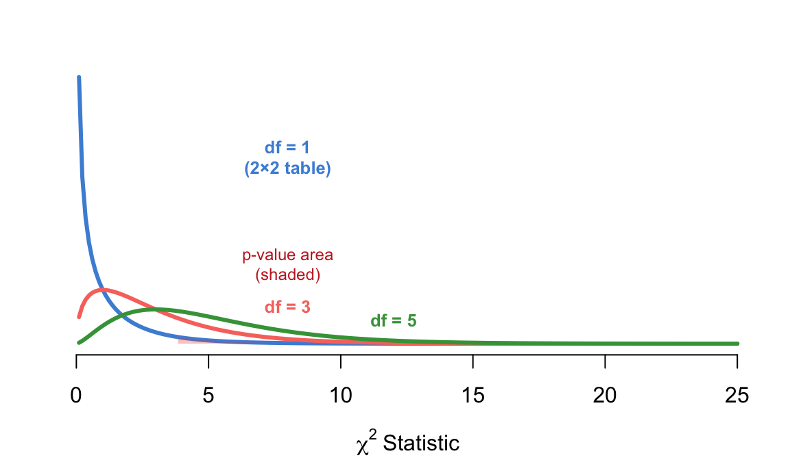
Chi-square distributions with different degrees of freedom. The test statistic is compared to the appropriate curve to find the p-value (shaded tail area).

Figure 7.1: Chi-square distributions with different degrees of freedom. The test statistic is compared to the appropriate curve to find the p-value (shaded tail area).

The p-value is the area under the curve to the right of your observed $\chi^2$ statistic. A larger $\chi^2$ pushes further into the right tail, producing a smaller p-value. This is the same logic you learned in Chapter 5 — just with a different distribution.

How does a huge $\chi^2$ like 88.598 become a microscopic p-value like $2.2 \times 10^{-16}$? With 1 degree of freedom, a $\chi^2$ of just 3.84 already has p = 0.05 — that is the critical value. A $\chi^2$ of 88.6 is so far to the right that the tail area is astronomically tiny. The computer reports $2.2 \times 10^{-16}$ because that is approximately the smallest number R can represent before rounding to zero. The math is: the larger the $\chi^2$, the more the observed table deviates from independence, and the smaller the probability of seeing such a table by chance alone.

7.3.6 When to Use Chi-Square (and When Not To)

Use chi-square when: - Both variables are categorical (C→C). - You want to test whether they are associated (not independent) in the population. - You have enough data — ideally, all expected counts should be at least 5. If more than 20% of expected counts are below 5, chi-square may not be reliable.

Do NOT use chi-square when: - Your response is quantitative → use t-test (Ch 5), ANOVA (Ch 6), or regression (Ch 9). - Your explanatory variable is quantitative and response is quantitative → use correlation (Ch 8) or regression (Ch 9). - You have a 2×2 table and small expected counts — consider Fisher’s exact test (fisher.test()).

7.3.7 The Big Picture: Chi-Square in the Inference Family

Test	Variable Pair	$H_0$	R Function
t-test (Ch 5)	C→Q (2 groups)	$\mu_1 = \mu_2$	`t.test()`
ANOVA (Ch 6)	C→Q (3+ groups)	All $\mu$ equal	`aov()`
Chi-Square (Ch 7)	C→C	Variables independent	`chisq.test()`
Correlation (Ch 8)	Q→Q	$\rho = 0$	`cor.test()`

Notice the pattern: the test you use is determined entirely by the types of your two variables. This table will guide you through the rest of Part II.

7.4 Code

7.4.1 Step 1: State the Hypotheses

$H_0$: There is no relationship between major depression and nicotine dependence among young adult daily smokers. (They are independent.)

$H_a$: There is a relationship between major depression and nicotine dependence among young adult daily smokers. (They are not independent.)

7.4.2 Step 2: Choose the Test

Both variables are categorical (C→C). The appropriate test is the chi-square test of independence.

7.4.3 Step 3: Assess the Evidence

7.4.3.1 Running the Chi-Square Test

The R function is chisq.test(). It accepts a two-way table (created with table() or xtabs()):

# Chi-square test of independence — ← REPLACE: table(row_var, col_var)
# Build the contingency table
dep_tab <- table(nesarc$MajorDepression, nesarc$TobaccoDependence)

# Run the chi-square test
# correct = FALSE → standard chi-square (no continuity correction)
chisq.test(dep_tab, correct = FALSE)

## 
##  Pearson's Chi-squared test
## 
## data:  dep_tab
## X-squared = 88.598, df = 1, p-value < 2.2e-16

Let us walk through the output line by line:

data: dep_tab — confirms which table we are testing.

X-squared = 30.862 — the chi-square test statistic. This measures the total discrepancy between observed and expected counts. For a 2×2 table, a value of 30.86 is very large — strong evidence against $H_0$.

df = 1 — degrees of freedom. For a 2×2 table, $df = (2-1) \times (2-1) = 1$.

p-value = 2.757e-08 — this is $2.76 \times 10^{-8}$, or 0.0000000276. That is far below 0.05. If depression and nicotine dependence were truly independent in the population, the chance of seeing a table this extreme (or more) is about 3 in 100 million. The evidence against $H_0$ is overwhelming.

What does correct = FALSE do? By default, R applies Yates’ continuity correction to 2×2 tables. This correction subtracts 0.5 from each $|O - E|$ difference before squaring, which makes the test slightly more conservative — p-values become a bit larger. Statisticians disagree about whether this correction is necessary. Many modern textbooks recommend correct = FALSE, which runs the standard Pearson chi-square test without adjustment. If you forget and leave the default (correct = TRUE), your results for a 2×2 table will be slightly more conservative but still valid. The difference is usually small unless your sample is very small. For tables larger than 2×2, R ignores the correction regardless, so correct = FALSE is just good practice — it keeps your behavior consistent across all table sizes.

7.4.3.2 Expected Counts

You can extract the expected counts from the test result to see exactly what independence would predict:

# Extract expected counts — what we would see under H_0
# ← REPLACE: store your test result, then access $expected
chisq_result <- chisq.test(dep_tab, correct = FALSE)
chisq_result$expected    # the expected counts under independence

##                 
##                  No Dependence Nicotine Dependence
##   No Depression       380.8826            584.1174
##   Yes Depression      140.1174            214.8826

Compare these to the observed counts. Which cells have the largest discrepancies? In our data, the cell for “No Depression + Nicotine Dependence” has 546 observed vs. 593 expected (fewer than expected), while “Yes Depression + Nicotine Dependence” has 153 observed vs. 106 expected (more than expected). Depression is associated with more nicotine dependence than independence would predict.

7.4.3.3 Clean Output with `broom::tidy()`

For a report, you want a clean table — not the wall of text from chisq.test(). Just like in Chapter 5, broom::tidy() converts the output to a tidy data frame:

# Clean results table with broom::tidy() + knitr::kable()
# ← REPLACE: your table, your caption
chisq_result <- chisq.test(dep_tab, correct = FALSE)
tidy(chisq_result) %>%
  knitr::kable(digits = 3,
               caption = "Chi-Square Test: Depression vs. Nicotine Dependence")

Table 5.2: Chi-Square Test: Depression vs. Nicotine Dependence
statistic	p.value	parameter	method
88.598	0	1	Pearson’s Chi-squared test

The tidy output gives you statistic ($\chi^2$), p.value, parameter (df), and method. To pull out just the p-value programmatically:

# Extract just the p-value from the chi-square result
# ← REPLACE: your table to reuse the stored result from above
chisq_result$p.value   # p-value directly from the test object

## [1] 4.838608e-21

7.4.3.4 Visualizing the Relationship

A statistical test confirms the association exists — but a graph shows what the association looks like. The stacked bar chart (from Chapter 4) is the right visualization for C→C:

# Stacked bar chart — show proportions for each depression group
# ← REPLACE: x = your explanatory variable, fill = your response variable
ggplot(data = nesarc, aes(x = MajorDepression, fill = TobaccoDependence)) +
  geom_bar(position = "fill") +                    # bars stretched to 100%
  theme_bw() +                                     # clean black-and-white theme
  labs(x = "", y = "Proportion",                   # ← REPLACE: your axis labels
       title = "Nicotine Dependence by Depression Status",
       subtitle = expression(chi^2 ~ "= 30.86, df = 1, p < 0.001")) +
  scale_fill_manual(values = c("#619CFF", "#F8766D"),  # custom bar colors
                    name = "Nicotine\nDependence")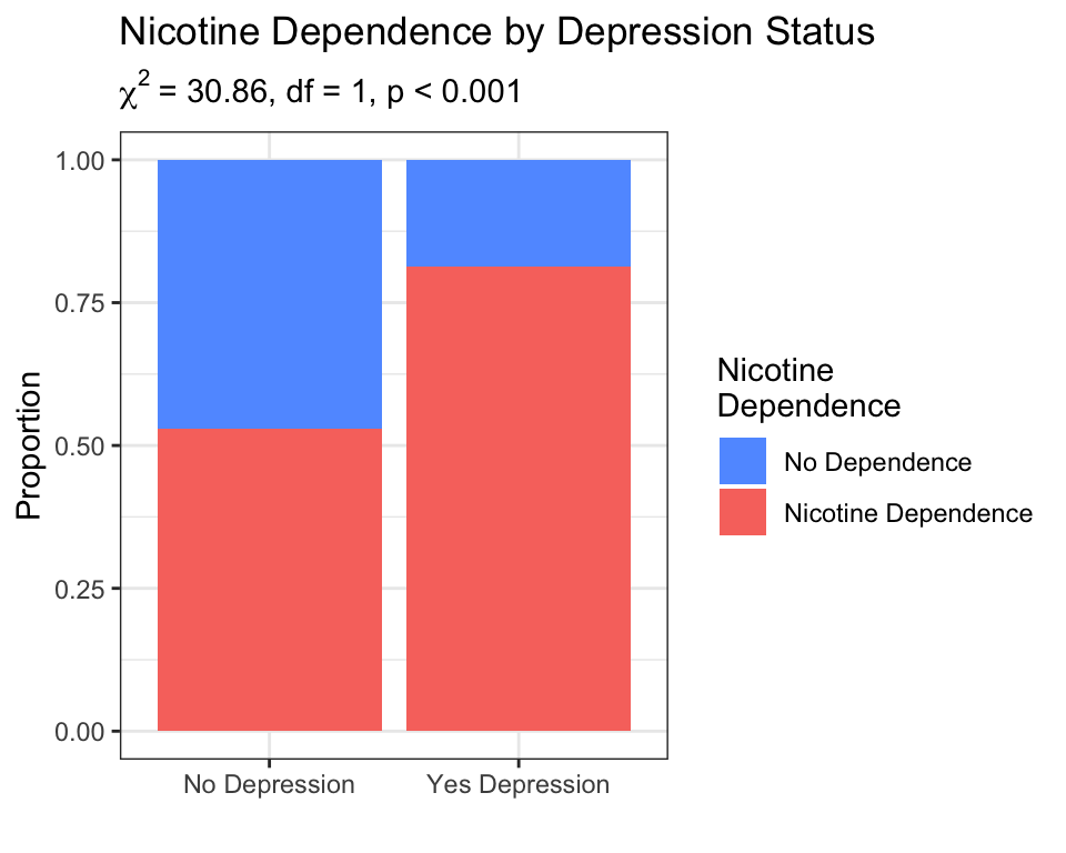

The red segment (nicotine dependence) is visibly taller in the “Yes Depression” bar. The chi-square test confirms this is not a chance pattern — it reflects a real association in the population.

7.4.4 Step 4: Draw a Conclusion

The p-value is $2.76 \times 10^{-8}$, which is far below 0.05. Therefore, we reject the null hypothesis. There is strong evidence that major depression and nicotine dependence are associated among young adult daily smokers. Specifically, those with major depression have a higher rate of nicotine dependence (76%) than those without depression (56%).

7.4.5 Writing Up Your Results

In a report or poster, write up a chi-square test in one sentence using this format:

A chi-square test of independence revealed a significant association between major depression and nicotine dependence among young adult daily smokers, $\chi^2$(1, N = 1,315) = 30.86, p < 0.001. Those with major depression were more likely to have nicotine dependence (76.3%) compared to those without depression (55.8%).

The format is: test name, $\chi^2$(df, N = sample size) = value, p-value. Then describe the direction of the association in plain language with the relevant percentages — readers need to know how the variables are related, not just that they are.

7.4.6 Example 2: More Than Two Categories — Post Hoc Tests

The chi-square test is not limited to 2×2 tables. What if your explanatory variable has more than two categories? Our NESARC data includes DailyCigsSmoked — a quantitative variable. But we can turn it into a categorical one by binning cigarettes per day into groups. This lets us ask:

Is the rate of nicotine dependence different across different levels of cigarette consumption?

First, let us create a categorical version of daily cigarettes. We will group smokers into five levels:

# Create a categorical variable from daily cigarette quantity
# ← REPLACE: your numeric variable and bin boundaries
nesarc$DCScat <- cut(nesarc$DailyCigsSmoked,
  breaks = c(0, 5, 10, 15, 20, 100),    # bin boundaries
  labels = c("1-5", "6-10", "11-15",    # ← REPLACE: your bin labels
             "16-20", ">20"),
  right = TRUE)                          # right-closed intervals: (0,5], (5,10], etc.

# Check the distribution across bins
table(nesarc$DCScat, useNA = "ifany")     # show counts including missing

## 
##   1-5  6-10 11-15 16-20   >20  <NA> 
##   249   477   134   368    87     5

cut() slices a numeric variable into bins. breaks defines the boundaries. labels assigns readable names. The result is a factor with ordered levels — perfect for a chi-square test.

Now run the chi-square test:

# Chi-square test — nicotine dependence across 5 cigarette quantity groups
# Use xtabs() with TobaccoDependence first → 2×5 table (rows=dependence, cols=cig groups)
# ← REPLACE: xtabs(~ response_var + explanatory_var, data = your_df)
dcscat_tab <- xtabs(~ TobaccoDependence + DCScat, data = nesarc)
dcscat_tab                                          # view the full 2×5 table

##                      DCScat
## TobaccoDependence     1-5 6-10 11-15 16-20 >20
##   No Dependence       130  210    43   114  20
##   Nicotine Dependence 119  267    91   254  67

# Run the chi-square test
chisq_dcscat <- chisq.test(dcscat_tab, correct = FALSE)
chisq_dcscat

## 
##  Pearson's Chi-squared test
## 
## data:  dcscat_tab
## X-squared = 45.159, df = 4, p-value = 3.685e-09

table() and xtabs() produce identical two-way frequency tables. The difference is purely in how you write them: table(nesarc$TobaccoDependence, nesarc$DCScat) uses $ to pull out columns, while xtabs(~ TobaccoDependence + DCScat, data = nesarc) uses a formula with ~ — the same formula style you have seen in t.test(), aov(), and datasummary(). The ~ means “model by” — read it as “cross-tabulate TobaccoDependence by DCScat.” Both functions feed into chisq.test() identically. Use whichever syntax feels more natural — if you are already writing formulas elsewhere in your code, xtabs() keeps your style consistent.

The p-value is well below 0.05 — there are significant differences in nicotine dependence rates across the five cigarette groups. But which groups differ from which? A significant chi-square tells you that at least one pair of groups differs, but not which ones. For that, you need post hoc tests.

7.4.6.1 Post Hoc Tests with Bonferroni Adjustment

When you compare multiple pairs of groups, you face the multiple comparisons problem. If you run 10 pairwise chi-square tests at $\alpha = 0.05$, you have a 40% chance of finding at least one “significant” result purely by chance — even if no real differences exist.

The Bonferroni adjustment fixes this: divide your significance level by the number of comparisons you make.

For our 5 cigarette groups, there are $\binom{5}{2} = 10$ possible pairwise comparisons. Our adjusted $\alpha$ is:

\[\alpha_{\text{adjusted}} = \frac{0.05}{10} = 0.005\]

Only p-values below 0.005 are considered statistically significant after the correction.

Is Bonferroni too strict? It can be — dividing $\alpha$ by the number of comparisons controls the chance of making any Type I error, which is a very conservative goal. When you have many comparisons (say, 20+), the adjusted threshold becomes so tiny that you may miss real effects. Researchers have developed less punishing alternatives: the Holm-Bonferroni method (slightly less strict, still controls the familywise error rate), and the Benjamini-Hochberg procedure (controls the false discovery rate — the proportion of your significant results that are actually false — allowing more discoveries). For this book, Bonferroni is the starting point because it is the simplest to understand and implement by hand. If your own project involves many comparisons, consider looking into Holm or Benjamini-Hochberg for a better balance between caution and discovery.

7.4.6.2 Running the Pairwise Comparisons

Here we run chi-square tests for all 10 pairs of cigarette groups. For each test, we subset the table to just two columns (two groups) and run chisq.test():

# Post hoc: 10 pairwise chi-square tests with Bonferroni adjustment
# ← REPLACE: dcscat_tab → your table, column indices → your group pairs
# Each test compares two of the 5 cigarette quantity groups
# Adjusted alpha = 0.05 / 10 = 0.005

# Pair 1: 1-5 vs 6-10
chisq.test(dcscat_tab[, c(1, 2)], correct = FALSE)

## 
##  Pearson's Chi-squared test
## 
## data:  dcscat_tab[, c(1, 2)]
## X-squared = 4.4003, df = 1, p-value = 0.03593

# Pair 2: 1-5 vs 11-15
chisq.test(dcscat_tab[, c(1, 3)], correct = FALSE)

## 
##  Pearson's Chi-squared test
## 
## data:  dcscat_tab[, c(1, 3)]
## X-squared = 14.238, df = 1, p-value = 0.000161

# Pair 3: 1-5 vs 16-20
chisq.test(dcscat_tab[, c(1, 4)], correct = FALSE)

## 
##  Pearson's Chi-squared test
## 
## data:  dcscat_tab[, c(1, 4)]
## X-squared = 28, df = 1, p-value = 1.213e-07

# Pair 4: 1-5 vs >20
chisq.test(dcscat_tab[, c(1, 5)], correct = FALSE)

## 
##  Pearson's Chi-squared test
## 
## data:  dcscat_tab[, c(1, 5)]
## X-squared = 22.275, df = 1, p-value = 2.362e-06

# Pair 5: 6-10 vs 11-15
chisq.test(dcscat_tab[, c(2, 3)], correct = FALSE)

## 
##  Pearson's Chi-squared test
## 
## data:  dcscat_tab[, c(2, 3)]
## X-squared = 6.1426, df = 1, p-value = 0.0132

# Pair 6: 6-10 vs 16-20
chisq.test(dcscat_tab[, c(2, 4)], correct = FALSE)

## 
##  Pearson's Chi-squared test
## 
## data:  dcscat_tab[, c(2, 4)]
## X-squared = 14.957, df = 1, p-value = 0.00011

# Pair 7: 6-10 vs >20
chisq.test(dcscat_tab[, c(2, 5)], correct = FALSE)

## 
##  Pearson's Chi-squared test
## 
## data:  dcscat_tab[, c(2, 5)]
## X-squared = 13.483, df = 1, p-value = 0.0002407

# Pair 8: 11-15 vs 16-20
chisq.test(dcscat_tab[, c(3, 4)], correct = FALSE)

## 
##  Pearson's Chi-squared test
## 
## data:  dcscat_tab[, c(3, 4)]
## X-squared = 0.056441, df = 1, p-value = 0.8122

# Pair 9: 11-15 vs >20
chisq.test(dcscat_tab[, c(3, 5)], correct = FALSE)

## 
##  Pearson's Chi-squared test
## 
## data:  dcscat_tab[, c(3, 5)]
## X-squared = 2.1439, df = 1, p-value = 0.1431

# Pair 10: 16-20 vs >20
chisq.test(dcscat_tab[, c(4, 5)], correct = FALSE)

## 
##  Pearson's Chi-squared test
## 
## data:  dcscat_tab[, c(4, 5)]
## X-squared = 2.1619, df = 1, p-value = 0.1415

That is a lot of output. Let us extract just the p-values from each test and compare them to the adjusted threshold:

# Extract all 10 p-values and compare to adjusted alpha = 0.005
# ← REPLACE: your table and group labels

# Define the 10 column pairs to compare
pairs <- list(c(1,2), c(1,3), c(1,4), c(1,5),
              c(2,3), c(2,4), c(2,5),
              c(3,4), c(3,5),
              c(4,5))

group_names <- c("1-5", "6-10", "11-15", "16-20", ">20")   # ← REPLACE: your labels
bonferroni_alpha <- 0.05 / length(pairs)                     # adjusted significance level

# Loop through each pair, run the test, and record the p-value
results <- data.frame(Comparison = character(10),
                      Chi_Sq = numeric(10),
                      P_Value = numeric(10),
                      Significant = character(10),
                      stringsAsFactors = FALSE)

for (i in 1:length(pairs)) {
  pair <- pairs[[i]]
  test <- chisq.test(dcscat_tab[, pair], correct = FALSE)
  results$Comparison[i] <- paste(group_names[pair[1]], "vs.", group_names[pair[2]])
  results$Chi_Sq[i] <- round(test$statistic, 2)
  results$P_Value[i] <- round(test$p.value, 5)
  results$Significant[i] <- ifelse(test$p.value < bonferroni_alpha, "Yes", "No")
}

# Display the summary table
results

##         Comparison Chi_Sq P_Value Significant
## 1     1-5 vs. 6-10   4.40 0.03593          No
## 2    1-5 vs. 11-15  14.24 0.00016         Yes
## 3    1-5 vs. 16-20  28.00 0.00000         Yes
## 4      1-5 vs. >20  22.28 0.00000         Yes
## 5   6-10 vs. 11-15   6.14 0.01320          No
## 6   6-10 vs. 16-20  14.96 0.00011         Yes
## 7     6-10 vs. >20  13.48 0.00024         Yes
## 8  11-15 vs. 16-20   0.06 0.81221          No
## 9    11-15 vs. >20   2.14 0.14314          No
## 10   16-20 vs. >20   2.16 0.14147          No

The Significant column shows which pairs differ after the Bonferroni correction. In our data, you will see that the lower cigarette groups (1-5, 6-10) differ significantly from the highest group (>20), but neighboring groups (like 11-15 vs. 16-20) are not significantly different. This pattern tells a story: nicotine dependence rates climb with cigarette consumption and then level off at the highest levels.

7.4.6.3 Visualizing Post Hoc Results

A stacked bar chart makes the pattern visually obvious:

# Stacked bar chart — nicotine dependence by cigarette quantity group
# ← REPLACE: x = your multi-category explanatory variable, fill = your response
ggplot(data = nesarc, aes(x = DCScat, fill = TobaccoDependence)) +
  geom_bar(position = "fill") +
  theme_bw() +
  labs(x = "Daily Cigarettes Smoked", y = "Proportion",
       title = "Nicotine Dependence by Cigarette Consumption Level",
       subtitle = expression(chi^2 ~ "test significant; bars with different letters differ (Bonferroni-adjusted)")) +
  scale_fill_manual(values = c("#619CFF", "#F8766D"),
                    name = "Nicotine\nDependence")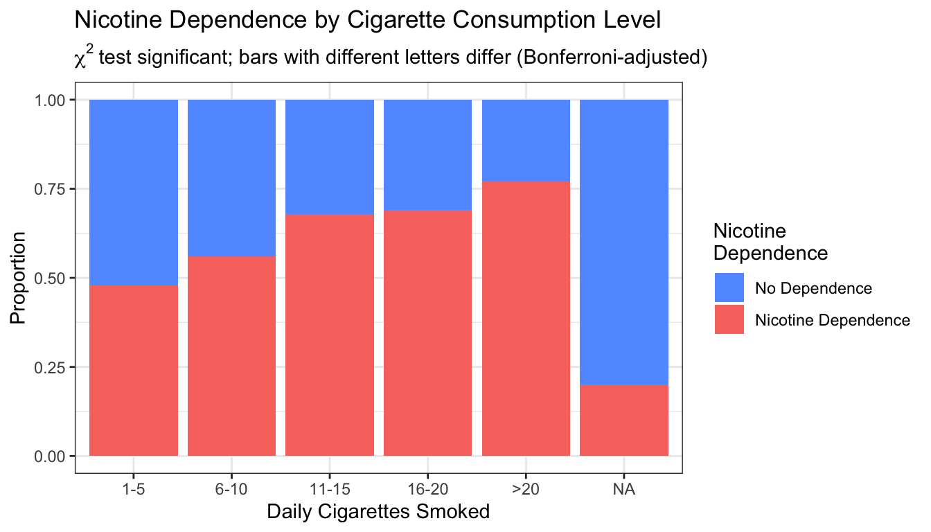

The red area (dependence) grows steadily from the “1-5” group to the “>20” group. The post hoc tests confirmed that the growth from the lowest to highest levels is statistically significant — not just visually apparent.

7.5 Interpretation

7.5.1 How to Read Chi-Square Output

For any chisq.test() output, find these three numbers:

What to Find	Where It Is	What It Tells You
$\chi^2$ statistic	`X-squared = ...`	How far the observed counts are from expected. Larger = stronger evidence against $H_0$.
Degrees of freedom	`df = ...`	$(r-1) \times (c-1)$. Determines the shape of the chi-square distribution used to calculate the p-value.
p-value	`p-value = ...`	If p < 0.05, reject $H_0$ — the variables are associated. If p ≥ 0.05, fail to reject $H_0$.

Golden rule for chi-square: the p-value tells you whether an association exists. The row proportions (from prop.table(tab, 1)) tell you what the association looks like and which direction it goes. Always report both.

7.5.2 Writing Up Chi-Square Results

The standard format for a chi-square write-up is:

A chi-square test of independence [was/was not] significant, $\chi^2$(df, N = sample_size) = value, p = X.XX. [Description of the association in plain language with relevant percentages.]

Examples:

Significant (our depression example): > A chi-square test of independence revealed a significant association between major depression and nicotine dependence, $\chi^2$(1, N = 1,315) = 30.86, p < 0.001. Young adult daily smokers with major depression had a higher rate of nicotine dependence (76.3%) than those without depression (55.8%).

Not significant: > A chi-square test of independence found no significant association between sex and nicotine dependence among young adult daily smokers, $\chi^2$(1, N = 1,315) = 1.23, p = 0.267. Rates of nicotine dependence were similar for females (58.9%) and males (60.2%).

With post hoc (significant omnibus test): > A chi-square test of independence revealed a significant association between cigarette consumption level and nicotine dependence, $\chi^2$(4, N = 1,258) = 45.16, p < 0.001. Post hoc pairwise comparisons with Bonferroni adjustment ($\alpha = 0.005$) showed that smokers in the 1-5 cigarettes per day group had significantly lower rates of nicotine dependence than those smoking 11 or more cigarettes per day. Rates did not differ significantly among the upper consumption groups (11-15, 16-20, >20 cigarettes per day).

7.5.3 Common Mistakes Students Make

Using chi-square when expected counts are too small. If more than 20% of your expected counts are below 5, the chi-square approximation may be unreliable. Check with chisq.test(tab)$expected. For 2×2 tables with small counts, use fisher.test() instead — Fisher’s exact test does not rely on large-sample approximations. Why is 5 the cutoff? It is a rule of thumb from simulation studies: statisticians found that the chi-square approximation (which uses a continuous distribution for discrete count data) breaks down when cells are too sparse. The number 5 emerged as the boundary where the approximation becomes trustworthy. Why not just always use Fisher’s test? Because Fisher’s test is computationally intensive for large tables — it calculates the exact probability of every possible table configuration, which grows exponentially with table dimensions. For a 5×5 table with a large sample, Fisher’s test could take minutes, while chi-square runs instantly. For 2×2 tables, Fisher’s is fast and many statisticians now recommend using it routinely regardless of expected counts.
Treating a 2×2 chi-square result as if it tells you the direction. The chi-square statistic is always positive — it measures total discrepancy, not direction. You must look at the row proportions to know how the variables are related.
Running many pairwise tests without adjusting $\alpha$. After a significant chi-square with 3+ groups, you must correct for multiple comparisons. The Bonferroni adjustment ($\alpha / \text{number of comparisons}$) is the simplest method. Without it, you will find “significant” differences that are actually just chance.
Confusing independence with no difference. Failing to reject $H_0$ does not prove the variables are independent. It only means the evidence was too weak to detect an association. With a small sample, even a real relationship may go undetected.
Forgetting to report the sample size. The chi-square statistic depends on the sample size. A $\chi^2$ of 10 in a sample of 200 is much more impressive than a $\chi^2$ of 10 in a sample of 10,000. Always include N in your write-up.
Ignoring the visual. Always graph your data before (and after) running a chi-square test. A stacked bar chart shows the association at a glance. The test formalizes what your eyes already see. If the graph and the test disagree, something is wrong — check your code.

7.5.4 What Comes Next

You have now learned the hypothesis test for the C→C variable pair. Combined with the t-test (C→Q, two groups) from Chapter 5 and ANOVA (C→Q, three+ groups) from Chapter 6, you can test associations for three of the four possible variable-type combinations.

The only combination remaining is Q→Q — when both your explanatory and response variables are quantitative. In that case, the question is not “are they associated?” but “how strongly are they linearly related?”

In Chapter 8 (Correlation), you will learn to quantify the strength and direction of a linear relationship between two quantitative variables. You will meet the correlation coefficient $r$, learn to test whether it differs from zero, and discover how $R^2$ measures the proportion of variance explained. The logic — state hypotheses, choose a test, assess evidence, draw a conclusion — stays exactly the same.

Test	Variable Pair	\(H_0\)	R Function
t-test (Ch 5)	C→Q (2 groups)	\(\mu_1 = \mu_2\)	`t.test()`
ANOVA (Ch 6)	C→Q (3+ groups)	All \(\mu\) equal	`aov()`
Chi-Square (Ch 7)	C→C	Variables independent	`chisq.test()`
Correlation (Ch 8)	Q→Q	\(\rho = 0\)	`cor.test()`

What to Find	Where It Is	What It Tells You
\(\chi^2\) statistic	`X-squared = ...`	How far the observed counts are from expected. Larger = stronger evidence against \(H_0\).
Degrees of freedom	`df = ...`	\((r-1) \times (c-1)\). Determines the shape of the chi-square distribution used to calculate the p-value.
p-value	`p-value = ...`	If p < 0.05, reject \(H_0\) — the variables are associated. If p ≥ 0.05, fail to reject \(H_0\).